Simulation with observer based state feedback of the string with mass model
Simulation environment
Simulation of the string with mass example, with flatness based state feedback and flatness based state observer (design + approximation), presented in [RW2018a].
References
Marcus Riesmeier and Frank Woittennek; Modale Approximation eines verteiltparametrischen Beobachters für das Modell der Saite mit Last. GMA Fachausschuss 1.40 „Systemtheorie und Regelungstechnik“, Salzburg, Austria, September 17-20, 2018.
- class FlatString(y0, y1, z0, z1, t0, dt, params)
Bases:
pyinduct.simulation.SimulationInputFlatness based feedforward for the “string with mass” model.
The flat output
 of this system is given by the mass position
at
of this system is given by the mass position
at  . This output will be transferred from y0 to y1
starting at t0, lasting dt seconds.
. This output will be transferred from y0 to y1
starting at t0, lasting dt seconds.- Parameters:
y0 (float) – Initial value for the flat output.
y1 (float) – Final value for the flat output.
z0 (float) – Position of the flat output (left side of the string).
z1 (float) – Position of the actuation (right side of the string).
t0 (float) – Time to start the transfer.
dt (float) – Duration of the transfer.
params (bunch) – Structure containing the physical parameters: * m: the mass * tau: the * sigma: the strings tension
- class Parameters
- class PgDataPlot(data)
Bases:
DataPlot,pyqtgraph.QtCore.QObjectBase class for all pyqtgraph plotting related classes.
- class SecondOrderFeedForward(desired_handle)
Bases:
pyinduct.examples.string_with_mass.system.pi.SimulationInputBase class for all objects that want to act as an input for the time-step simulation.
The calculated values for each time-step are stored in internal memory and can be accessed by
get_results()(after the simulation is finished).Note
Due to the underlying solver, this handle may get called with time arguments, that lie outside of the specified integration domain. This should not be a problem for a feedback controller but might cause problems for a feedforward or trajectory implementation.
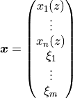
- class SwmBaseCanonicalFraction(functions, scalars)
Bases:
pyinduct.ComposedFunctionVectorImplementation of composite function vector
 .
.
- derive(order)
Basic implementation of derive function.
Empty implementation, overwrite to use this functionality. For an example implementation see
Function- Parameters:
order (
numbers.Number) – derivative order- Returns:
derived object
- Return type:
- evaluation_hint(values)
If evaluation can be accelerated by using special properties of a function, this function can be overwritten to performs that computation. It gets passed an array of places where the caller wants to evaluate the function and should return an array of the same length, containing the results.
Note
This implementation just calls the normal evaluation hook.
- Parameters:
values – places to be evaluated at
- Returns:
Evaluation results.
- Return type:
numpy.ndarray
- get_member(idx)
Getter function to access members. Empty function, overwrite to implement custom functionality. For an example implementation see
FunctionNote
Empty function, overwrite to implement custom functionality.
- Parameters:
idx – member index
- static scalar_product(left, right)
- scalar_product_hint()
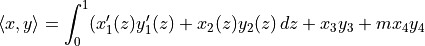
Scalar product for the canonical form of the string with mass system:
- Returns:
Scalar product function handle wrapped inside a list.
- Return type:
list(callable)
- class SwmBaseFraction(functions, scalars)
Bases:
pyinduct.ComposedFunctionVectorImplementation of composite function vector
.- derive(order)
Basic implementation of derive function.
Empty implementation, overwrite to use this functionality. For an example implementation see
Function- Parameters:
order (
numbers.Number) – derivative order- Returns:
derived object
- Return type:
- evaluation_hint(values)
If evaluation can be accelerated by using special properties of a function, this function can be overwritten to performs that computation. It gets passed an array of places where the caller wants to evaluate the function and should return an array of the same length, containing the results.
Note
This implementation just calls the normal evaluation hook.
- Parameters:
values – places to be evaluated at
- Returns:
Evaluation results.
- Return type:
numpy.ndarray
- get_member(idx)
Getter function to access members. Empty function, overwrite to implement custom functionality. For an example implementation see
FunctionNote
Empty function, overwrite to implement custom functionality.
- Parameters:
idx – member index
- l2_scalar_product = True
- static scalar_product(left, right)
- scalar_product_hint()
Scalar product for the string with mass system:
- Returns:
Scalar product function handle wrapped inside a list.
- Return type:
list(callable)
- class SwmObserverError(control_law, smooth=None)
Bases:
pyinduct.examples.string_with_mass.system.pi.StateFeedbackFor a smooth fade-in of the observer error.
- Parameters:
control_law (
WeakFormulation) – Function handle that calculates the control output if provided with correct weights.smooth (array-like) – Arguments for
SmoothTransition
- class SwmPgAnimatedPlot(data, title='', refresh_time=40, replay_gain=1, save_pics=False, create_video=False, labels=None)
Bases:
pyinduct.visualization.PgDataPlotAnimation for the string with mass example. Compare with
PgAnimatedPlot.- Parameters:
data ((iterable of)
EvalData) – results to animatetitle (basestring) – window title
refresh_time (int) – time in msec to refresh the window must be greater than zero
replay_gain (float) – values above 1 acc- and below 1 decelerate the playback process, must be greater than zero
save_pics (bool) –
labels –
Return:
- property exported_files
- apply_control_mode(sys_fem_lbl, sys_modal_lbl, obs_fem_lbl, obs_modal_lbl, mode)
- approximate_controller(sys_lbl, modal_lbl)
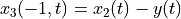
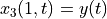
- build_canonical_weak_formulation(obs_lbl, spatial_domain, u, obs_err, name='system')
Observer canonical form of the string with mass example
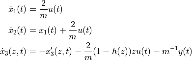
Boundary condition
Weak formulation
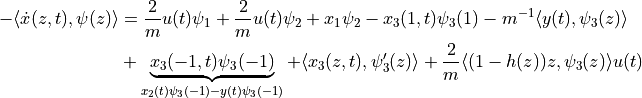
Output equation
- Parameters:
sys_approx_label (string) – Shapefunction label for system approximation.
obs_approx_label (string) – Shapefunction label for observer approximation.
input_vector (
pyinduct.simulation.SimulationInputVector) – Holds the input variable.params –
Python class with the members:
m (mass)
k1_ob, k2_ob, alpha_ob (observer parameters)
- Returns:
Observer
- Return type:
pyinduct.simulation.Observer
- build_controller(sys_lbl, ctrl_lbl)
The control law from [Woi2012] (equation 29)
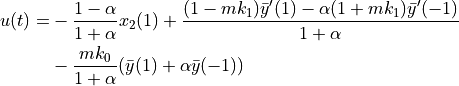
is simply tipped off in this function, whereas
![\begin{align*}
\bar{y}(\theta) &= \left\{\begin{array}{lll}
\xi_1 + m(1-e^{-\theta/m})\xi_2 +
\int_0^\theta (1-e^{-(\theta-\tau)/m}) (x_1'(\tau) + x_2(\tau)) \, dz
& \forall & \theta\in[-1, 0) \\
\xi_1 + m(e^{\theta/m}-1)\xi_2 +
\int_0^\theta (e^{(\theta-\tau)/m}-1) (x_1'(-\tau) - x_2(-\tau)) \, dz
& \forall & \theta\in[0, 1]
\end{array}\right. \\
\bar{y}'(\theta) &= \left\{\begin{array}{lll}
e^{-\theta/m}\xi_2 + \frac{1}{m}
\int_0^\theta e^{-(\theta-\tau)/m} (x_1'(\tau) + x_2(\tau)) \, dz
& \forall & \theta\in[-1, 0) \\
e^{\theta/m}\xi_2 + \frac{1}{m}
\int_0^\theta e^{(\theta-\tau)/m} (x_1'(-\tau) - x_2(-\tau)) \, dz
& \forall & \theta\in[0, 1].
\end{array}\right.
\end{align*}](../_images/math/be998dc785825f37aa71f37d82bee3eb43ae5578.png)
- Parameters:
approx_label (string) – Shapefunction label for approximation.
- Returns:
Control law
- Return type:
- build_fem_bases(base_lbl, n1, n2, cf_base_lbl, ncf, modal_base_lbl)
- build_modal_bases(base_lbl, n, cf_base_lbl, ncf)
- build_original_weak_formulation(sys_lbl, spatial_domain, u, name='system')
Projection (see
SwmBaseFraction.scalar_product_hint()
Boundary conditions

Implemented

- Parameters:
sys_lbl (str) – Base label
spatial_domain (
Domain) – Spatial domain of the system.name (str) – Name of the system.
- Returns:
- check_eigenvalues(sys_fem_lbl, obs_fem_lbl, obs_modal_lbl, ceq, ss)
- ctrl_gain
- find_eigenvalues(n)
- flatness_based_controller(x2_plus1, y_bar_plus1, y_bar_minus1, dz_y_bar_plus1, dz_y_bar_minus1, name)
- get_colors(cnt, scheme='tab10', samples=10)
Create a list of colors.
- Parameters:
cnt (int) – Number of colors in the list.
scheme (str) – Mpl color scheme to use.
samples (cnt) – Number of samples to take from the scheme before starting from the beginning.
- Returns:
List of np.Array holding the rgb values.
- get_modal_base_for_ctrl_approximation()
- get_primal_eigenvector(according_paper=False)
- init_observer_gain(sys_fem_lbl, sys_modal_lbl, obs_fem_lbl, obs_modal_lbl)
- integrate_function(func, interval)
Numerically integrate a function on a given interval using
complex_quadrature().- Parameters:
func (callable) – Function to integrate.
interval (list of tuples) – List of (start, end) values of the intervals to integrate on.
- Returns:
(Result of the Integration, errors that occurred during the integration).
- Return type:
tuple
- obs_gain
- ocf_inverse_state_transform(org_state)
Transformation of the the state
 into the coordinates of the observer canonical form
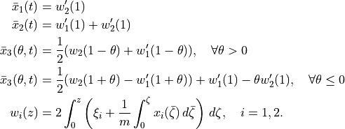
- Parameters:
org_state (
SwmBaseFraction) – State- Returns:
Transformation
- Return type:
SwmBaseCanonicalFraction
- param
- plot_eigenvalues(eigenvalues, return_figure=False)
- pprint(expression='\n\n\n')
- register_evp_base(base_lbl, eigenvectors, sp_var, domain)
- run(show_plots)
- scale_equation_term_list(eqt_list, factor)
Temporary function, as long
EquationTermcan only be scaled individually.- Parameters:
eqt_list (list) – List of
EquationTerm’sfactor (numbers.Number) – Scale factor.
- Returns:
Scaled copy of
EquationTerm’s (eqt_list).
- sort_eigenvalues(eigenvalues)
- subs_list = [()]
- sym
Weak formulations and definition of the bases
- class Parameters
- class PgDataPlot(data)
Bases:
DataPlot,pyqtgraph.QtCore.QObjectBase class for all pyqtgraph plotting related classes.
- class SwmBaseCanonicalFraction(functions, scalars)
Bases:
pyinduct.ComposedFunctionVectorImplementation of composite function vector
.- derive(order)
Basic implementation of derive function.
Empty implementation, overwrite to use this functionality. For an example implementation see
Function- Parameters:
order (
numbers.Number) – derivative order- Returns:
derived object
- Return type:
- evaluation_hint(values)
If evaluation can be accelerated by using special properties of a function, this function can be overwritten to performs that computation. It gets passed an array of places where the caller wants to evaluate the function and should return an array of the same length, containing the results.
Note
This implementation just calls the normal evaluation hook.
- Parameters:
values – places to be evaluated at
- Returns:
Evaluation results.
- Return type:
numpy.ndarray
- get_member(idx)
Getter function to access members. Empty function, overwrite to implement custom functionality. For an example implementation see
FunctionNote
Empty function, overwrite to implement custom functionality.
- Parameters:
idx – member index
- static scalar_product(left, right)
- scalar_product_hint()
Scalar product for the canonical form of the string with mass system:
- Returns:
Scalar product function handle wrapped inside a list.
- Return type:
list(callable)
- class SwmBaseFraction(functions, scalars)
Bases:
pyinduct.ComposedFunctionVectorImplementation of composite function vector
.- derive(order)
Basic implementation of derive function.
Empty implementation, overwrite to use this functionality. For an example implementation see
Function- Parameters:
order (
numbers.Number) – derivative order- Returns:
derived object
- Return type:
- evaluation_hint(values)
If evaluation can be accelerated by using special properties of a function, this function can be overwritten to performs that computation. It gets passed an array of places where the caller wants to evaluate the function and should return an array of the same length, containing the results.
Note
This implementation just calls the normal evaluation hook.
- Parameters:
values – places to be evaluated at
- Returns:
Evaluation results.
- Return type:
numpy.ndarray
- get_member(idx)
Getter function to access members. Empty function, overwrite to implement custom functionality. For an example implementation see
FunctionNote
Empty function, overwrite to implement custom functionality.
- Parameters:
idx – member index
- l2_scalar_product = True
- static scalar_product(left, right)
- scalar_product_hint()
Scalar product for the string with mass system:
- Returns:
Scalar product function handle wrapped inside a list.
- Return type:
list(callable)
- class SwmPgAnimatedPlot(data, title='', refresh_time=40, replay_gain=1, save_pics=False, create_video=False, labels=None)
Bases:
pyinduct.visualization.PgDataPlotAnimation for the string with mass example. Compare with
PgAnimatedPlot.- Parameters:
data ((iterable of)
EvalData) – results to animatetitle (basestring) – window title
refresh_time (int) – time in msec to refresh the window must be greater than zero
replay_gain (float) – values above 1 acc- and below 1 decelerate the playback process, must be greater than zero
save_pics (bool) –
labels –
Return:
- property exported_files
- build_canonical_weak_formulation(obs_lbl, spatial_domain, u, obs_err, name='system')
Observer canonical form of the string with mass example
Boundary condition
Weak formulation
Output equation
- Parameters:
sys_approx_label (string) – Shapefunction label for system approximation.
obs_approx_label (string) – Shapefunction label for observer approximation.
input_vector (
pyinduct.simulation.SimulationInputVector) – Holds the input variable.params –
Python class with the members:
m (mass)
k1_ob, k2_ob, alpha_ob (observer parameters)
- Returns:
Observer
- Return type:
pyinduct.simulation.Observer
- build_fem_bases(base_lbl, n1, n2, cf_base_lbl, ncf, modal_base_lbl)
- build_modal_bases(base_lbl, n, cf_base_lbl, ncf)
- build_original_weak_formulation(sys_lbl, spatial_domain, u, name='system')
Projection (see
SwmBaseFraction.scalar_product_hint()Boundary conditions
Implemented
- Parameters:
sys_lbl (str) – Base label
spatial_domain (
Domain) – Spatial domain of the system.name (str) – Name of the system.
- Returns:
- check_eigenvalues(sys_fem_lbl, obs_fem_lbl, obs_modal_lbl, ceq, ss)
- ctrl_gain
- find_eigenvalues(n)
- get_colors(cnt, scheme='tab10', samples=10)
Create a list of colors.
- Parameters:
cnt (int) – Number of colors in the list.
scheme (str) – Mpl color scheme to use.
samples (cnt) – Number of samples to take from the scheme before starting from the beginning.
- Returns:
List of np.Array holding the rgb values.
- get_modal_base_for_ctrl_approximation()
- get_primal_eigenvector(according_paper=False)
- integrate_function(func, interval)
Numerically integrate a function on a given interval using
complex_quadrature().- Parameters:
func (callable) – Function to integrate.
interval (list of tuples) – List of (start, end) values of the intervals to integrate on.
- Returns:
(Result of the Integration, errors that occurred during the integration).
- Return type:
tuple
- obs_gain
- param
- plot_eigenvalues(eigenvalues, return_figure=False)
- pprint(expression='\n\n\n')
- register_evp_base(base_lbl, eigenvectors, sp_var, domain)
- sort_eigenvalues(eigenvalues)
- subs_list = [()]
- sym
State feedback control
- class Parameters
- class PgDataPlot(data)
Bases:
DataPlot,pyqtgraph.QtCore.QObjectBase class for all pyqtgraph plotting related classes.
- class SecondOrderFeedForward(desired_handle)
Bases:
pyinduct.examples.string_with_mass.system.pi.SimulationInputBase class for all objects that want to act as an input for the time-step simulation.
The calculated values for each time-step are stored in internal memory and can be accessed by
get_results()(after the simulation is finished).Note
Due to the underlying solver, this handle may get called with time arguments, that lie outside of the specified integration domain. This should not be a problem for a feedback controller but might cause problems for a feedforward or trajectory implementation.
- class SwmBaseCanonicalFraction(functions, scalars)
Bases:
pyinduct.ComposedFunctionVectorImplementation of composite function vector
.- derive(order)
Basic implementation of derive function.
Empty implementation, overwrite to use this functionality. For an example implementation see
Function- Parameters:
order (
numbers.Number) – derivative order- Returns:
derived object
- Return type:
- evaluation_hint(values)
If evaluation can be accelerated by using special properties of a function, this function can be overwritten to performs that computation. It gets passed an array of places where the caller wants to evaluate the function and should return an array of the same length, containing the results.
Note
This implementation just calls the normal evaluation hook.
- Parameters:
values – places to be evaluated at
- Returns:
Evaluation results.
- Return type:
numpy.ndarray
- get_member(idx)
Getter function to access members. Empty function, overwrite to implement custom functionality. For an example implementation see
FunctionNote
Empty function, overwrite to implement custom functionality.
- Parameters:
idx – member index
- static scalar_product(left, right)
- scalar_product_hint()
Scalar product for the canonical form of the string with mass system:
- Returns:
Scalar product function handle wrapped inside a list.
- Return type:
list(callable)
- class SwmBaseFraction(functions, scalars)
Bases:
pyinduct.ComposedFunctionVectorImplementation of composite function vector
.- derive(order)
Basic implementation of derive function.
Empty implementation, overwrite to use this functionality. For an example implementation see
Function- Parameters:
order (
numbers.Number) – derivative order- Returns:
derived object
- Return type:
- evaluation_hint(values)
If evaluation can be accelerated by using special properties of a function, this function can be overwritten to performs that computation. It gets passed an array of places where the caller wants to evaluate the function and should return an array of the same length, containing the results.
Note
This implementation just calls the normal evaluation hook.
- Parameters:
values – places to be evaluated at
- Returns:
Evaluation results.
- Return type:
numpy.ndarray
- get_member(idx)
Getter function to access members. Empty function, overwrite to implement custom functionality. For an example implementation see
FunctionNote
Empty function, overwrite to implement custom functionality.
- Parameters:
idx – member index
- l2_scalar_product = True
- static scalar_product(left, right)
- scalar_product_hint()
Scalar product for the string with mass system:
- Returns:
Scalar product function handle wrapped inside a list.
- Return type:
list(callable)
- class SwmObserverError(control_law, smooth=None)
Bases:
pyinduct.examples.string_with_mass.system.pi.StateFeedbackFor a smooth fade-in of the observer error.
- Parameters:
control_law (
WeakFormulation) – Function handle that calculates the control output if provided with correct weights.smooth (array-like) – Arguments for
SmoothTransition
- class SwmPgAnimatedPlot(data, title='', refresh_time=40, replay_gain=1, save_pics=False, create_video=False, labels=None)
Bases:
pyinduct.visualization.PgDataPlotAnimation for the string with mass example. Compare with
PgAnimatedPlot.- Parameters:
data ((iterable of)
EvalData) – results to animatetitle (basestring) – window title
refresh_time (int) – time in msec to refresh the window must be greater than zero
replay_gain (float) – values above 1 acc- and below 1 decelerate the playback process, must be greater than zero
save_pics (bool) –
labels –
Return:
- property exported_files
- apply_control_mode(sys_fem_lbl, sys_modal_lbl, obs_fem_lbl, obs_modal_lbl, mode)
- approximate_controller(sys_lbl, modal_lbl)
- build_canonical_weak_formulation(obs_lbl, spatial_domain, u, obs_err, name='system')
Observer canonical form of the string with mass example
Boundary condition
Weak formulation
Output equation
- Parameters:
sys_approx_label (string) – Shapefunction label for system approximation.
obs_approx_label (string) – Shapefunction label for observer approximation.
input_vector (
pyinduct.simulation.SimulationInputVector) – Holds the input variable.params –
Python class with the members:
m (mass)
k1_ob, k2_ob, alpha_ob (observer parameters)
- Returns:
Observer
- Return type:
pyinduct.simulation.Observer
- build_controller(sys_lbl, ctrl_lbl)
The control law from [Woi2012] (equation 29)
is simply tipped off in this function, whereas
- Parameters:
approx_label (string) – Shapefunction label for approximation.
- Returns:
Control law
- Return type:
- build_fem_bases(base_lbl, n1, n2, cf_base_lbl, ncf, modal_base_lbl)
- build_modal_bases(base_lbl, n, cf_base_lbl, ncf)
- build_original_weak_formulation(sys_lbl, spatial_domain, u, name='system')
Projection (see
SwmBaseFraction.scalar_product_hint()Boundary conditions
Implemented
- Parameters:
sys_lbl (str) – Base label
spatial_domain (
Domain) – Spatial domain of the system.name (str) – Name of the system.
- Returns:
- check_eigenvalues(sys_fem_lbl, obs_fem_lbl, obs_modal_lbl, ceq, ss)
- ctrl_gain
- find_eigenvalues(n)
- flatness_based_controller(x2_plus1, y_bar_plus1, y_bar_minus1, dz_y_bar_plus1, dz_y_bar_minus1, name)
- get_colors(cnt, scheme='tab10', samples=10)
Create a list of colors.
- Parameters:
cnt (int) – Number of colors in the list.
scheme (str) – Mpl color scheme to use.
samples (cnt) – Number of samples to take from the scheme before starting from the beginning.
- Returns:
List of np.Array holding the rgb values.
- get_modal_base_for_ctrl_approximation()
- get_primal_eigenvector(according_paper=False)
- init_observer_gain(sys_fem_lbl, sys_modal_lbl, obs_fem_lbl, obs_modal_lbl)
- integrate_function(func, interval)
Numerically integrate a function on a given interval using
complex_quadrature().- Parameters:
func (callable) – Function to integrate.
interval (list of tuples) – List of (start, end) values of the intervals to integrate on.
- Returns:
(Result of the Integration, errors that occurred during the integration).
- Return type:
tuple
- obs_gain
- ocf_inverse_state_transform(org_state)
Transformation of the the state
into the coordinates of the observer canonical form- Parameters:
org_state (
SwmBaseFraction) – State- Returns:
Transformation
- Return type:
SwmBaseCanonicalFraction
- param
- plot_eigenvalues(eigenvalues, return_figure=False)
- pprint(expression='\n\n\n')
- register_evp_base(base_lbl, eigenvectors, sp_var, domain)
- scale_equation_term_list(eqt_list, factor)
Temporary function, as long
EquationTermcan only be scaled individually.- Parameters:
eqt_list (list) – List of
EquationTerm’sfactor (numbers.Number) – Scale factor.
- Returns:
Scaled copy of
EquationTerm’s (eqt_list).
- sort_eigenvalues(eigenvalues)
- subs_list = [()]
- sym