Simulation of the Euler-Bernoulli Beam
In this example, the hyperbolic equation of an euler bernoulli beam, clamped
at one side is considered.
The domain of the vertical beam excitation  is regarded to be
![[0, 1] \times \mathbb{R}^+](../_images/math/74927ef48953e33428d329a926880d4d006c055c.png) .
.
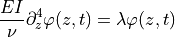
The governing equation reads:
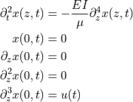
With the E-module  , the second moment of area
  and the
specific density
and the
specific density  .
In this example, the input
.
In this example, the input  mimics the force impulse occurring if
the beam is hit by a hammer.
mimics the force impulse occurring if
the beam is hit by a hammer.
Spatial disretization
For further analysis let 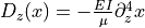 denote
the spatial operator and
denote
the spatial operator and
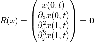
denote the boundary operator.
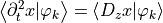
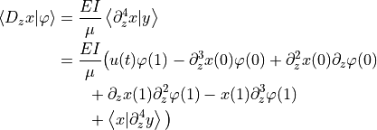
Repeated partial integration of the expression
![\begin{align*}
\left< D_z x | \varphi \right>
&= \frac{EI}{\mu} \left< \partial^4_z x | y \right>\\
&= \frac{EI}{\mu} \left(
\left[\partial^3_z x \varphi \right]_0^1
-\left[\partial^2_z x \partial_z\varphi \right]_0^1
\left[\partial^1_z x \partial^2_z\varphi \right]_0^1
-\left[ x \partial^3_z\varphi \right]_0^1
\right)\\
&\quad + \frac{EI}{\mu} \left< x | \partial^4_z y \right>
\end{align*}](../_images/math/d06ef601a014ae8f03f0159084d6130225371ba8.png)
and application of the boundary conditions shows that
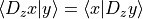 if
if
 . Therefore, the spatial operator is self-adjoint.
Modal Analysis
Since the operator is self-adjoined, the eigenvectors of the operator generate a orthonormal basis, which can be used for the approximation.
Hence, the problem to solve reads:
Which is achieved by choosing
where 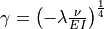 .
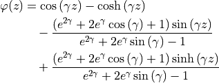
This is done in
.
This is done in calc_eigen() .
Using this basis, the approximation
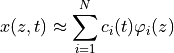
is introduced.
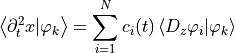
Projecting the equation on the basis of eigenvectors
 yields
for every  . Substituting the approximation leads to
where the application of  and the inner product can be swapped since
is a bounded operator.
Finally, using the solution of the eigen problem yields
and the inner product can be swapped since
is a bounded operator.
Finally, using the solution of the eigen problem yields
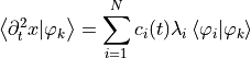
which simplifies to
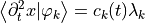
since, due to orthonormality,  is
zero for all
is
zero for all  and
and  for
for  .
.
Performing the same steps for the left-hand side yields:
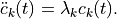
Thus, the ordinary differential equation system
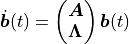
with the new state vector

the integrator chain  and eigenvalue matrix
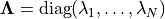 is
derived.
Since the resulting system is autonomous, apart from interesting simulations,
not much can be done fro a control perspective.
is
derived.
Since the resulting system is autonomous, apart from interesting simulations,
not much can be done fro a control perspective.
Alternative Variant
Using the weak formulation, which is gained by projecting the original equation on a set of test functions and fully shifting the spatial operator onto the test functions and substituting the boundary conditions
and inserting the modal approximation from above, the system can be simulated
for every arbitrary input . Note that this approximation converges
over the whole spatial domain, but not punctually, since using the eigenvectors
 but
but  .
.
source code:
"""
This example simulates an euler-bernoulli beam, please refer to the
documentation for an exhaustive explanation.
"""

import numpy as np
import sympy as sp
import pyinduct as pi
from matplotlib import pyplot as plt


class ImpulseExcitation(pi.SimulationInput):
    """
    Simulate that the free end of the beam is hit by a hammer
    """

    def _calc_output(self, **kwargs):
        t = kwargs["time"]
        a = 1/20
        value = 100 / (a * np.sqrt(np.pi)) * np.exp(-((t-1)/a)**2)
        return dict(output=value)


def calc_eigen(order, l_value, EI, mu, der_order=4, debug=False):
    r"""
    Solve the eigenvalue problem and return the eigenvectors

    Args:
        order: Approximation order.
        l_value: Length of the spatial domain.
        EI: Product of e-module and second moment of inertia.
        mu: Specific density.
        der_order: Required derivative order of the generated functions.

    Returns:
        pi.Base: Modal base.
    """
    C, D, E, F = sp.symbols("C D E F")
    gamma, l = sp.symbols("gamma l")
    z = sp.symbols("z")

    eig_func = (C*sp.cos(gamma*z)
                + D*sp.sin(gamma*z)
                + E*sp.cosh(gamma*z)
                + F*sp.sinh(gamma*z))

    bcs = [eig_func.subs(z, 0),
           eig_func.diff(z, 1).subs(z, 0),
           eig_func.diff(z, 2).subs(z, l),
           eig_func.diff(z, 3).subs(z, l),
           ]
    e_sol = sp.solve(bcs[0], E)[0]
    f_sol = sp.solve(bcs[1], F)[0]
    new_bcs = [bc.subs([(E, e_sol), (F, f_sol)]) for bc in bcs[2:]]
    d_sol = sp.solve(new_bcs[0], D)[0]
    char_eq = new_bcs[1].subs([(D, d_sol), (l, l_value), (C, 1)])
    char_func = sp.lambdify(gamma, char_eq, modules="numpy")

    def char_wrapper(z):
        try:
            return char_func(z)
        except FloatingPointError:
            return 1

    grid = np.linspace(-1, 30, num=1000)
    roots = pi.find_roots(char_wrapper, grid, n_roots=order)
    if debug:
        pi.visualize_roots(roots, grid, char_func)

    # build eigenvectors
    eig_vec = eig_func.subs([(E, e_sol),
                             (F, f_sol),
                             (D, d_sol),
                             (l, l_value),
                             (C, 1)])

    # print(sp.latex(eig_vec))

    # build derivatives
    eig_vec_derivatives = [eig_vec]
    for i in range(der_order):
        eig_vec_derivatives.append(eig_vec_derivatives[-1].diff(z, 1))

    # construct functions
    eig_fractions = []
    for root in roots:
        # localize and lambdify
        callbacks = [sp.lambdify(z, vec.subs(gamma, root), modules="numpy")
                     for vec in eig_vec_derivatives]

        frac = pi.Function(domain=(0, l_value),
                           eval_handle=callbacks[0],
                           derivative_handles=callbacks[1:])
        frac.eigenvalue = - root**4 * EI / mu
        eig_fractions.append(frac)

    eig_base = pi.Base(eig_fractions)
    normed_eig_base = pi.normalize_base(eig_base)

    if debug:
        pi.visualize_functions(eig_base.fractions)
        pi.visualize_functions(normed_eig_base.fractions)

    return normed_eig_base


def run(show_plots):
    sys_name = 'euler bernoulli beam'

    # domains
    spat_bounds = (0, 1)
    spat_domain = pi.Domain(bounds=spat_bounds, num=101)
    temp_domain = pi.Domain(bounds=(0, 10), num=1000)

    if 0:
        # physical properties
        height = .1  # [m]
        width = .1  # [m]
        e_module = 210e9  # [Pa]
        EI = 210e9 * (width * height**3)/12
        mu = 1e6  # [kg/m]
    else:
        # normed properties
        EI = 1e0
        mu = 1e0

    # define approximation bases
    if 0:
        # somehow, fem is still problematic
        approx_base = pi.LagrangeNthOrder.cure_interval(spat_domain,
                                                        order=4)
        approx_lbl = "complete_base"
    else:
        approx_base = calc_eigen(7, 1, EI, mu)
        approx_lbl = "eig_base"

    pi.register_base(approx_lbl, approx_base)

    # system definition

    u = ImpulseExcitation("Hammer")
    x = pi.FieldVariable(approx_lbl)
    phi = pi.TestFunction(approx_lbl)

    weak_form = pi.WeakFormulation([
        pi.ScalarTerm(pi.Product(pi.Input(u), phi(1)), scale=EI),
        pi.ScalarTerm(pi.Product(x.derive(spat_order=3)(0), phi(0)),
                      scale=-EI),
        pi.ScalarTerm(pi.Product(x.derive(spat_order=2)(0), phi.derive(1)(0)),
                      scale=EI),
        pi.ScalarTerm(pi.Product(x.derive(spat_order=1)(1), phi.derive(2)(1)),
                      scale=EI),
        pi.ScalarTerm(pi.Product(x(1), phi.derive(3)(1)),
                      scale=-EI),
        pi.IntegralTerm(pi.Product(x, phi.derive(4)),
                        spat_bounds,
                        scale=EI),
        pi.IntegralTerm(pi.Product(x.derive(temp_order=2), phi),
                        spat_bounds,
                        scale=mu),
    ], name=sys_name)

    # initial conditions
    init_form = pi.ConstantFunction(0, domain=spat_bounds)
    init_form_dt = pi.ConstantFunction(0, domain=spat_bounds)
    initial_conditions = [init_form, init_form_dt]

    # simulation
    with np.errstate(under="ignore"):
        eval_data = pi.simulate_system(weak_form,
                                       initial_conditions,
                                       temp_domain,
                                       spat_domain,
                                       settings=dict(name="vode",
                                                     method="bdf",
                                                     order=5,
                                                     nsteps=1e8,
                                                     max_step=temp_domain.step))
    pi.tear_down([approx_lbl])

    # recover the input trajectory
    u_data = u.get_results(eval_data[0].input_data[0], as_eval_data=True)

    # visualization
    if show_plots:
        plt.plot(u_data.input_data[0], u_data.output_data)
        win1 = pi.PgAnimatedPlot(eval_data,
                                 labels=dict(left='x(z,t)', bottom='z'))
        pi.show()


if __name__ == "__main__":
    run(True)