Core¶

In the Core module you can find all basic classes and functions which form the backbone of the toolbox.

class ApproximationBasis[source]¶

Base class for an approximation basis.

An approximation basis is formed by some objects on which given distributed variables may be projected.

abstract function_space_hint()[source]¶: Hint that returns properties that characterize the functional space of the fractions. It can be used to determine if function spaces match.

Note

Overwrite to implement custom functionality.

is_compatible_to(other)[source]¶

Helper functions that checks compatibility between two approximation bases.

In this case compatibility is given if the two bases live in the same function space.

Parameters:: other (Approximation Base) – Approximation basis to compare with.

Returns: True if bases match, False if they do not.

abstract scalar_product_hint()[source]¶: Hint that returns steps for scalar product calculation with elements of this base.

Note

Overwrite to implement custom functionality.

class Base(fractions, matching_base_lbls=None, intermediate_base_lbls=None)[source]¶

Bases: ApproximationBasis

Base class for approximation bases.

In general, a Base is formed by a certain amount of BaseFractions and therefore forms finite-dimensional subspace of the distributed problem’s domain. Most of the time, the user does not need to interact with this class.

Parameters:

fractions (iterable of BaseFraction) – List, array or dict of BaseFraction’s
matching_base_lbls (list of str) – List of labels from exactly matching bases, for which no transformation is necessary. Useful for transformations from bases that ‘live’ in different function spaces but evolve with the same time dynamic/coefficients (e.g. modal bases).
intermediate_base_lbls (list of str) – If it is certain that this base instance will be asked (as destination base) to return a transformation to a source base, whose implementation is cumbersome, its label can be provided here. This will trigger the generation of the transformation using build-in features. The algorithm, implemented in get_weights_transformation is then called again with the intermediate base as destination base and the ‘old’ source base. With this technique arbitrary long transformation chains are possible, if the provided intermediate bases again define intermediate bases.

_get_intermediate_transform(info, inter_lbl)[source]¶

static _transformation_factory(info, equivalent=False)[source]¶

derive(order)[source]¶

Basic implementation of derive function. Empty implementation, overwrite to use this functionality.

Parameters:: order (numbers.Number) – derivative order
Returns:: derived object
Return type:: Base

function_space_hint()[source]¶: Hint that returns properties that characterize the functional space of the fractions. It can be used to determine if function spaces match.

Note

Overwrite to implement custom functionality.

get_attribute(attr)[source]¶

Retrieve an attribute from the fractions of the base.

Parameters:: attr (str) – Attribute to query the fractions for.
Returns:: Array of len(fractions) holding the attributes. With None entries if the attribute is missing.
Return type:: np.ndarray

raise_to(power)[source]¶

Factory method to obtain instances of this base, raised by the given power.

Parameters:: power – power to raise the basis onto.

scalar_product_hint()[source]¶: Hint that returns steps for scalar product calculation with elements of this base.

Note

Overwrite to implement custom functionality.

scale(factor)[source]¶

Return a scaled instance of this base.

If factor is iterable, each element will be scaled independently. Otherwise, a common scaling is applied to all fractions.

Parameters:: factor – Single factor or iterable of factors (float or callable) to scale this base with.

transformation_hint(info)[source]¶

Method that provides a information about how to transform weights from one BaseFraction into another.

In Detail this function has to return a callable, which will take the weights of the source- and return the weights of the target system. It may have keyword arguments for other data which is required to perform the transformation. Information about these extra keyword arguments should be provided in form of a dictionary whose keys are keyword arguments of the returned transformation handle.

Note

This implementation covers the most basic case, where the two BaseFraction’s are of same type. For any other case it will raise an exception. Overwrite this Method in your implementation to support conversion between bases that differ from yours.

Parameters:: info – TransformationInfo
Raises:: NotImplementedError –
Returns:: Transformation handle

class BaseFraction(members)[source]¶

Abstract base class representing a basis that can be used to describe functions of several variables.

abstract _apply_operator(operator, additive=False)[source]¶

Return a new base fraction with the given operator applied.

Parameters:

operator – Object that can be applied to the base fraction.
additive – Define if the given operator is additive. Default: False. For an additive operator G and two base fractions f, h the relation G(f + h) = G(f) + G(h) holds. If the operator is not additive the derivatives will be discarded.

abstract add_neutral_element()[source]¶

Return the neutral element of addition for this object.

In other words: self + ret_val == self.

conj()[source]¶: Return the complex conjugated base fraction.

derive(order)[source]¶

Basic implementation of derive function.

Empty implementation, overwrite to use this functionality. For an example implementation see Function

Parameters:: order (numbers.Number) – derivative order
Returns:: derived object
Return type:: BaseFraction

evaluation_hint(values)[source]¶

If evaluation can be accelerated by using special properties of a function, this function can be overwritten to performs that computation. It gets passed an array of places where the caller wants to evaluate the function and should return an array of the same length, containing the results.

Note

This implementation just calls the normal evaluation hook.

Parameters:: values – places to be evaluated at
Returns:: Evaluation results.
Return type:: numpy.ndarray

function_space_hint()[source]¶: Empty Hint that can return properties which uniquely define the function space of the BaseFraction.

Note

Overwrite to implement custom functionality. For an example implementation see Function.

abstract get_member(idx)[source]¶

Getter function to access members. Empty function, overwrite to implement custom functionality. For an example implementation see Function

Note

Empty function, overwrite to implement custom functionality.

Parameters:: idx – member index

imag()[source]¶: Return the imaginary port of the base fraction.

abstract mul_neutral_element()[source]¶

Return the neutral element of multiplication for this object.

In other words: self * ret_val == self.

raise_to(power)[source]¶

Raises this fraction to the given power.

Parameters:: power (numbers.Number) – power to raise the fraction onto
Returns:: raised fraction

real()[source]¶: Return the real part of the base fraction.

scalar_product_hint()[source]¶: Empty Hint that can return steps for scalar product calculation.

Note

Overwrite to implement custom functionality. For an example implementation see Function

abstract scale(factor)[source]¶

Factory method to obtain instances of this base fraction, scaled by the given factor. Empty function, overwrite to implement custom functionality. For an example implementation see Function.

Parameters:: factor – Factor to scale the vector.

class ComposedFunctionVector(functions, scalars)[source]¶

Bases: BaseFraction

Implementation of composite function vector $\boldsymbol{x}$ .

$\boldsymbol{x} = \begin{pmatrix} x_1(z) \\ \vdots \\ x_n(z) \\ \xi_1 \\ \vdots \\ \xi_m \\ \end{pmatrix}$

_apply_operator(operator, additive=False)[source]¶: Return a new composed function vector with the given operator applied. See docstring of BaseFraction._apply_operator().

add_neutral_element()[source]¶

Create neutral element of addition that is compatible to this object.

Returns: Comp. Function Vector with constant functions returning 0 and: scalars of value 0.

function_space_hint()[source]¶

Return the hint that this function is an element of the an scalar product space which is uniquely defined by

the scalar product ComposedFunctionVector.scalar_product()

len(self.members["funcs"]) functions

and len(self.members["scalars"]) scalars.

get_member(idx)[source]¶

Getter function to access members. Empty function, overwrite to implement custom functionality. For an example implementation see Function

Note

Empty function, overwrite to implement custom functionality.

Parameters:: idx – member index

mul_neutral_element()[source]¶

Create neutral element of multiplication that is compatible to this object.

Returns: Comp. Function Vector with constant functions returning 1 and: scalars of value 1.

scalar_product_hint()[source]¶: Empty Hint that can return steps for scalar product calculation.

Note

Overwrite to implement custom functionality. For an example implementation see Function

scale(factor)[source]¶

Factory method to obtain instances of this base fraction, scaled by the given factor. Empty function, overwrite to implement custom functionality. For an example implementation see Function.

Parameters:: factor – Factor to scale the vector.

class ConstantComposedFunctionVector(func_constants, scalar_constants, **func_kwargs)[source]¶

Bases: ComposedFunctionVector

Constant composite function vector $\boldsymbol{x}$ .

$\boldsymbol{x} = \begin{pmatrix} z \mapsto x_1(z) = c_1 \\ \vdots \\ z \mapsto x_n(z) = c_n \\ d_1 \\ \vdots \\ c_n \\ \end{pmatrix}$

Parameters:

func_constants (array-like) – Constants for the functions.
scalar_constants (array-like) – The scalar constants.
**func_kwargs – Keyword args that are passed to the ConstantFunction.

class ConstantFunction(constant, **kwargs)[source]¶

Bases: Function

A Function that returns a constant value.

This function can be differentiated without limits.

Parameters:: constant (number) – value to return
Keyword Arguments:: **kwargs – All other kwargs get passed to Function.

_constant_function_handle(z)[source]¶

derive(order=1)[source]¶

Spatially derive this Function.

This is done by neglecting order derivative handles and to select handle $\text{order} - 1$ as the new evaluation_handle.

Parameters:

order (int) – the amount of derivations to perform

Raises:

TypeError – If order is not of type int.
ValueError – If the requested derivative order is higher than the provided one.

Returns:

Function the derived function.

class Domain(bounds=None, num=None, step=None, points=None)[source]¶

Bases: object

Helper class that manages ranges for data evaluation, containing parameters.

Parameters:

bounds (tuple) – Interval bounds.
num (int) – Number of points in interval.
step (numbers.Number) – Distance between points (if homogeneous).
points (array_like) – Points themselves.

Note

If num and step are given, num will take precedence.

property bounds¶

property ndim¶

property points¶

property step¶

class EvalData(input_data, output_data, input_labels=None, input_units=None, enable_extrapolation=False, fill_axes=False, fill_value=None, name=None)[source]¶

This class helps managing any kind of result data.

The data gained by evaluation of a function is stored together with the corresponding points of its evaluation. This way all data needed for plotting or other postprocessing is stored in one place. Next to the points of the evaluation the names and units of the included axes can be stored. After initialization an interpolator is set up, so that one can interpolate in the result data by using the overloaded __call__() method.

Parameters:

input_data – (List of) array(s) holding the axes of a regular grid on which the evaluation took place.
output_data – The result of the evaluation.

Keyword Arguments:

input_labels – (List of) labels for the input axes.
input_units – (List of) units for the input axes.
name – Name of the generated data set.
fill_axes – If the dimension of output_data is higher than the length of the given input_data list, dummy entries will be appended until the required dimension is reached.
enable_extrapolation (bool) – If True, internal interpolators will allow extrapolation. Otherwise, the last giben value will be repeated for 1D cases and the result will be padded with zeros for cases > 1D.
fill_value – If invalid data is encountered, it will be replaced with this value before interpolation is performed.

Examples

When instantiating 1d EvalData objects, the list can be omitted

>>> axis = Domain((0, 10), 5)
>>> data = np.random.rand(5,)
>>> e_1d = EvalData(axis, data)

For other cases, input_data has to be a list

>>> axis1 = Domain((0, 0.5), 5)
>>> axis2 = Domain((0, 1), 11)
>>> data = np.random.rand(5, 11)
>>> e_2d = EvalData([axis1, axis2], data)

Adding two Instances (if the boundaries fit, the data will be interpolated on the more coarse grid.) Same goes for subtraction and multiplication.

>>> e_1 = EvalData(Domain((0, 10), 5), np.random.rand(5,))
>>> e_2 = EvalData(Domain((0, 10), 10), 100*np.random.rand(5,))
>>> e_3 = e_1 + e_2
>>> e_3.output_data.shape
(5,)

Interpolate in the output data by calling the object

>>> e_4 = EvalData(np.array(range(5)), 2*np.array(range(5))))
>>> e_4.output_data
array([0, 2, 4, 6, 8])
>>> e_5 = e_4([2, 5])
>>> e_5.output_data
array([4, 8])
>>> e_5.output_data.size
2

one may also give a slice

>>> e_6 = e_4(slice(1, 5, 2))
>>> e_6.output_data
array([2., 6.])
>>> e_5.output_data.size
2

For multi-dimensional interpolation a list has to be provided

>>> e_7 = e_2d([[.1, .5], [.3, .4, .7)])
>>> e_7.output_data.shape
(2, 3)

abs()[source]¶

Get the absolute value of the elements form self.output_data .

Returns:: EvalData with self.input_data and output_data as result of absolute value calculation.

add(other, from_left=True)[source]¶

Perform the element-wise addition of the output_data arrays from self and other

This method is used to support addition by implementing __add__ (fromLeft=True) and __radd__(fromLeft=False)). If other** is a EvalData, the input_data lists of self and other are adjusted using adjust_input_vectors() The summation operation is performed on the interpolated output_data. If other is a numbers.Number it is added according to numpy’s broadcasting rules.

Parameters:

other (numbers.Number or EvalData) – Number or EvalData object to add to self.
from_left (bool) – Perform the addition from left if True or from right if False.

Returns:

EvalData with adapted input_data and output_data as result of the addition.

adjust_input_vectors(other)[source]¶

Check the the inputs vectors of self and other for compatibility (equivalence) and harmonize them if they are compatible.

The compatibility check is performed for every input_vector in particular and examines whether they share the same boundaries. and equalize to the minimal discretized axis. If the amount of discretization steps between the two instances differs, the more precise discretization is interpolated down onto the less precise one.

Parameters:

other (EvalData) – Other EvalData class.

Returns:

(list) - New common input vectors.
(numpy.ndarray) - Interpolated self output_data array.
(numpy.ndarray) - Interpolated other output_data array.

Return type:

tuple

interpolate(interp_axis)[source]¶

Main interpolation method for output_data.

If one of the output dimensions is to be interpolated at one single point, the dimension of the output will decrease by one.

Parameters:

interp_axis (list(list)) – axis positions in the form
1D (-) – axis with axis=[1,2,3]
2D (-) – [axis1, axis2] with axis1=[1,2,3] and axis2=[0,1,2,3,4]

Returns:

EvalData with interp_axis as new input_data and interpolated output_data.

matmul(other, from_left=True)[source]¶

Perform the matrix multiplication of the output_data arrays from self and other .

This method is used to support matrix multiplication (@) by implementing __matmul__ (from_left=True) and __rmatmul__(from_left=False)). If other** is a EvalData, the input_data lists of self and other are adjusted using adjust_input_vectors(). The matrix multiplication operation is performed on the interpolated output_data. If other is a numbers.Number it is handled according to numpy’s broadcasting rules.

Parameters:

other (EvalData) – Object to multiply with.
from_left (boolean) – Matrix multiplication from left if True or from right if False.

Returns:

EvalData with adapted input_data and output_data as result of matrix multiplication.

mul(other, from_left=True)[source]¶

Perform the element-wise multiplication of the output_data arrays from self and other .

This method is used to support multiplication by implementing __mul__ (from_left=True) and __rmul__(from_left=False)). If other** is a EvalData, the input_data lists of self and other are adjusted using adjust_input_vectors(). The multiplication operation is performed on the interpolated output_data. If other is a numbers.Number it is handled according to numpy’s broadcasting rules.

Parameters:

other (numbers.Number or EvalData) – Factor to multiply with.
boolean (from_left) – Multiplication from left if True or from right if False.

Returns:

EvalData with adapted input_data and output_data as result of multiplication.

sqrt()[source]¶

Radicate the elements form self.output_data element-wise.

Returns:: EvalData with self.input_data and output_data as result of root calculation.

sub(other, from_left=True)[source]¶

Perform the element-wise subtraction of the output_data arrays from self and other .

This method is used to support subtraction by implementing __sub__ (from_left=True) and __rsub__(from_left=False)). If other** is a EvalData, the input_data lists of self and other are adjusted using adjust_input_vectors(). The subtraction operation is performed on the interpolated output_data. If other is a numbers.Number it is handled according to numpy’s broadcasting rules.

Parameters:

other (numbers.Number or EvalData) – Number or EvalData object to subtract.
from_left (boolean) – Perform subtraction from left if True or from right if False.

Returns:

EvalData with adapted input_data and output_data as result of subtraction.

class Function(eval_handle, domain=(-np.inf, np.inf), nonzero=(-np.inf, np.inf), derivative_handles=None)[source]¶

Bases: BaseFraction

Most common instance of a BaseFraction. This class handles all tasks concerning derivation and evaluation of functions. It is used broad across the toolbox and therefore incorporates some very specific attributes. For example, to ensure the accurateness of numerical handling functions may only evaluated in areas where they provide nonzero return values. Also their domain has to be taken into account. Therefore the attributes domain and nonzero are provided.

To save implementation time, ready to go version like LagrangeFirstOrder are provided in the pyinduct.simulation module.

For the implementation of new shape functions subclass this implementation or directly provide a callable eval_handle and callable derivative_handles if spatial derivatives are required for the application.

Parameters:

eval_handle (derivatives of) – Callable object that can be evaluated.
domain (nonzero output. Must be a subset of) – Domain on which the eval_handle is defined.
nonzero (tuple) – Region in which the eval_handle will return
domain –
derivative_handles (list) – List of callable(s) that contain
eval_handle –

_apply_operator(operator, additive=False)[source]¶: Return a new function with the given operator applied. See docstring of BaseFraction._apply_operator().

_check_domain(values)[source]¶

Checks if values fit into domain.

Parameters:: values (array_like) – Point(s) where function shall be evaluated.
Raises:: ValueError – If values exceed the domain.

add_neutral_element()[source]¶

Return the neutral element of addition for this object.

In other words: self + ret_val == self.

property derivative_handles¶

derive(order=1)[source]¶

Spatially derive this Function.

This is done by neglecting order derivative handles and to select handle $\text{order} - 1$ as the new evaluation_handle.

Parameters:

order (int) – the amount of derivations to perform

Raises:

TypeError – If order is not of type int.
ValueError – If the requested derivative order is higher than the provided one.

Returns:

Function the derived function.

static from_data(x, y, **kwargs)[source]¶

Create a Function based on discrete data by interpolating.

The interpolation is done by using interp1d from scipy, the kwargs will be passed.

Parameters:

x (array-like) – Places where the function has been evaluated .
y (array-like) – Function values at x.
**kwargs – all kwargs get passed to Function .

Returns:

An interpolating function.

Return type:

Function

property function_handle¶

function_space_hint()[source]¶: Return the hint that this function is an element of the an scalar product space which is uniquely defined by the scalar product scalar_product_hint().

Note

If you are working on different function spaces, you have to overwrite this hint in order to provide more properties which characterize your specific function space. For example the domain of the functions.

get_member(idx)[source]¶

Implementation of the abstract parent method.

Since the Function has only one member (itself) the parameter idx is ignored and self is returned.

Parameters:: idx – ignored.
Returns:: self

mul_neutral_element()[source]¶

Return the neutral element of multiplication for this object.

In other words: self * ret_val == self.

raise_to(power)[source]¶

Raises the function to the given power.

Warning

Derivatives are lost after this action is performed.

Parameters:: power (numbers.Number) – power to raise the function to
Returns:: raised function

scalar_product_hint()[source]¶: Return the hint that the _dot_product_l2() has to calculated to gain the scalar product.

scale(factor)[source]¶

Factory method to scale a Function.

Parameters:: factor – numbers.Number or a callable.

class Parameters(**kwargs)[source]¶

Handy class to collect system parameters. This class can be instantiated with a dict, whose keys will the become attributes of the object. (Bunch approach)

Parameters:: kwargs – parameters

class StackedBase(base_info)[source]¶

Bases: ApproximationBasis

Implementation of a basis vector that is obtained by stacking different bases onto each other. This typically occurs when the bases of coupled systems are joined to create a unified system.

Parameters:

base_info (OrderedDict) –

Dictionary with base_label as keys and dictionaries holding information about the bases as values. In detail, these Information must contain:

sys_name (str): Name of the system the base is associated with.

order (int): Highest temporal derivative order with which the
base shall be represented in the stacked base.

base (ApproximationBase): The actual basis.

function_space_hint()[source]¶: Hint that returns properties that characterize the functional space of the fractions. It can be used to determine if function spaces match.

Note

Overwrite to implement custom functionality.

is_compatible_to(other)[source]¶

Helper functions that checks compatibility between two approximation bases.

In this case compatibility is given if the two bases live in the same function space.

Parameters:: other (Approximation Base) – Approximation basis to compare with.

Returns: True if bases match, False if they do not.

scalar_product_hint()[source]¶: Hint that returns steps for scalar product calculation with elements of this base.

Note

Overwrite to implement custom functionality.

abstract scale(factor)[source]¶

transformation_hint(info)[source]¶

If info.src_lbl is a member, just return it, using to correct derivative transformation, otherwise return None

Parameters:: info (TransformationInfo) – Information about the requested transformation.
Returns:: transformation handle

class TransformationInfo[source]¶

Structure that holds information about transformations between different bases.

This class serves as an easy to use structure to aggregate information, describing transformations between different BaseFraction s. It can be tested for equality to check the equity of transformations and is hashable which makes it usable as dictionary key to cache different transformations.

src_lbl¶

label of source basis

Type:: str

dst_lbl¶

label destination basis

Type:: str

src_base¶

source basis in form of an array of the source Fractions

Type:: numpy.ndarray

dst_base¶

destination basis in form of an array of the destination Fractions

Type:: numpy.ndarray

src_order¶: available temporal derivative order of source weights

dst_order¶: needed temporal derivative order for destination weights

as_tuple()[source]¶

mirror()[source]¶: Factory method, that creates a new TransformationInfo object by mirroring src and dst terms. This helps handling requests to different bases.

back_project_from_base(weights, base)[source]¶

Build evaluation handle for a distributed variable that was approximated as a set of weights om a certain base.

Parameters:

weights (numpy.ndarray) – Weight vector.
base (ApproximationBase) – Base to be used for the projection.

Returns:

evaluation handle

calculate_base_transformation_matrix(src_base, dst_base, scalar_product=None)[source]¶

Calculates the transformation matrix $V$ , so that the a set of weights, describing a function in the src_base will express the same function in the dst_base, while minimizing the reprojection error. An quadratic error is used as the error-norm for this case.

Warning

This method assumes that all members of the given bases have the same type and that their BaseFraction s, define compatible scalar products.

Raises:

TypeError – If given bases do not provide an scalar_product_hint() method.

Parameters:

src_base (ApproximationBase) – Current projection base.
dst_base (ApproximationBase) – New projection base.
scalar_product (list of callable) – Callbacks for product calculation. Defaults to scalar_product_hint from src_base.

Returns:

Transformation matrix $V$ .

Return type:

numpy.ndarray

calculate_expanded_base_transformation_matrix(src_base, dst_base, src_order, dst_order, use_eye=False)[source]¶

Constructs a transformation matrix $\bar V$ from basis given by src_base to basis given by dst_base that also transforms all temporal derivatives of the given weights.

See:: calculate_base_transformation_matrix() for further details.

Parameters:

dst_base (ApproximationBase) – New projection base.
src_base (ApproximationBase) – Current projection base.
src_order – Temporal derivative order available in src_base.
dst_order – Temporal derivative order needed in dst_base.
use_eye (bool) – Use identity as base transformation matrix. (For easy selection of derivatives in the same base)

Raises:

ValueError – If destination needs a higher derivative order than source can provide.

Returns:

Transformation matrix

Return type:

numpy.ndarray

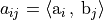
calculate_scalar_matrix(values_a, values_b)[source]¶

Convenience version of py:function:calculate_scalar_product_matrix with numpy.multiply() hardcoded as scalar_product_handle.

Parameters:

values_a (numbers.Number or numpy.ndarray) – (array of) value(s) for rows
values_b (numbers.Number or numpy.ndarray) – (array of) value(s) for columns

Returns:

Matrix containing the pairwise products of the elements from values_a and values_b.

Return type:

numpy.ndarray

calculate_scalar_product_matrix(base_a, base_b, scalar_product=None, optimize=True)[source]¶

Calculates a matrix $A$ , whose elements are the scalar products of each element from base_a and base_b, so that $a_{ij} = \langle \mathrm{a}_i\,,\: \mathrm{b}_j\rangle$ .

Parameters:

base_a (ApproximationBase) – Basis a
base_b (ApproximationBase) – Basis b
scalar_product – (List of) function objects that are passed the members of the given bases as pairs. Defaults to the scalar product given by base_a
optimize (bool) – Switch to turn on the symmetry based speed up. For development purposes only.

Returns:

matrix $A$

Return type:

numpy.ndarray

change_projection_base(src_weights, src_base, dst_base)[source]¶

Converts given weights that form an approximation using src_base to the best possible fit using dst_base.

Parameters:

src_weights (numpy.ndarray) – Vector of numbers.
src_base (ApproximationBase) – The source Basis.
dst_base (ApproximationBase) – The destination Basis.

Returns:

target weights

Return type:

numpy.ndarray

complex_quadrature(func, a, b, **kwargs)[source]¶

Wraps the scipy.qaudpack routines to handle complex valued functions.

Parameters:

func (callable) – function
a (numbers.Number) – lower limit
b (numbers.Number) – upper limit
**kwargs – Arbitrary keyword arguments for desired scipy.qaudpack routine.

Returns:

(real part, imaginary part)

Return type:

tuple

complex_wrapper(func)[source]¶

Wraps complex valued functions into two-dimensional functions. This enables the root-finding routine to handle it as a vectorial function.

Parameters:: func (callable) – Callable that returns a complex result.
Returns:: function handle, taking x = (re(x), im(x) and returning [re(func(x), im(func(x)].
Return type:: two-dimensional, callable

domain_intersection(first, second)[source]¶

Calculate intersection(s) of two domains.

Parameters:

first (set) – (Set of) tuples defining the first domain.
second (set) – (Set of) tuples defining the second domain.

Returns:

Intersection given by (start, end) tuples.

Return type:

set

domain_simplification(domain)[source]¶

Simplify a domain, given by possibly overlapping subdomains.

Parameters:: domain (set) – Set of tuples, defining the (start, end) points of the subdomains.
Returns:: Simplified domain.
Return type:: list

dot_product(first, second)[source]¶

Calculate the inner product of two vectors. Uses numpy.inner but with complex conjugation of the second argument.

Parameters:

first (numpy.ndarray) – first vector
second (numpy.ndarray) – second vector

Returns:

inner product

dot_product_l2(first, second)[source]¶

Calculate the inner product on L2.

Given two functions $\varphi(z)$ (first) and $\psi(z)$ (second) this functions calculates

$\left< \varphi(z) | \psi(z) \right> = \int\limits_{\Gamma_0}^{\Gamma_1} \varphi(\zeta) \bar\psi(\zeta) \,\textup{d}\zeta \:.$

Parameters:

first (Function) – first function $\varphi(z)$
second (Function) – second function $\psi(z)$

Returns:

inner product

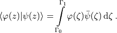
find_roots(function, grid, n_roots=None, rtol=1e-05, atol=1e-08, cmplx=False, sort_mode='norm')[source]¶

Searches n_roots roots of the function $f(\boldsymbol{x})$ on the given grid and checks them for uniqueness with aid of rtol.

In Detail scipy.optimize.root() is used to find initial candidates for roots of $f(\boldsymbol{x})$ . If a root satisfies the criteria given by atol and rtol it is added. If it is already in the list, a comprehension between the already present entries’ error and the current error is performed. If the newly calculated root comes with a smaller error it supersedes the present entry.

Raises:

ValueError – If the demanded amount of roots can’t be found.

Parameters:

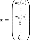
function (callable) – Function handle for math:f(boldsymbol{x}) whose roots shall be found.
grid (list) – Grid to use as starting point for root detection. The $i$ th element of this list provides sample points for the $i$ th parameter of $\boldsymbol{x}$ .
n_roots (int) – Number of roots to find. If none is given, return all roots that could be found in the given area.
rtol – Tolerance to be exceeded for the difference of two roots to be unique: $f(r1) - f(r2) > \textrm{rtol}$ .
atol – Absolute tolerance to zero: $f(x^0) < \textrm{atol}$ .
cmplx (bool) – Set to True if the given function is complex valued.
sort_mode (str) – Specify tho order in which the extracted roots shall be sorted. Default “norm” sorts entries by their $l_2$ norm, while “component” will sort them in increasing order by every component.

Returns:

numpy.ndarray of roots; sorted in the order they are returned by $f(\boldsymbol{x})$ .

generic_scalar_product(b1, b2=None, scalar_product=None)[source]¶

Calculates the pairwise scalar product between the elements of the ApproximationBase b1 and b2.

Parameters:

b1 (ApproximationBase) – first basis
b2 (ApproximationBase) – second basis, if omitted defaults to b1
scalar_product (list of callable) – Callbacks for product calculation. Defaults to scalar_product_hint from b1.

Note

If b2 is omitted, the result can be used to normalize b1 in terms of its scalar product.

get_base(label)[source]¶

Retrieve registered set of initial functions by their label.

Parameters:: label (str) – String, label of functions to retrieve.
Returns:: initial_functions

get_transformation_info(source_label, destination_label, source_order=0, destination_order=0)[source]¶

Provide the weights transformation from one/source base to another/destination base.

Parameters:

source_label (str) – Label from the source base.
destination_label (str) – Label from the destination base.
source_order – Order from the available time derivative of the source weights.
destination_order – Order from the desired time derivative of the destination weights.

Returns:

Transformation info object.

Return type:

TransformationInfo

get_weight_transformation(info)[source]¶

Create a handle that will transform weights from info.src_base into weights for info-dst_base while paying respect to the given derivative orders.

This is accomplished by recursively iterating through source and destination bases and evaluating their transformation_hints.

Parameters:: info (TransformationInfo) – information about the requested transformation.
Returns:: transformation function handle
Return type:: callable

integrate_function(func, interval)[source]¶

Numerically integrate a function on a given interval using complex_quadrature().

Parameters:

func (callable) – Function to integrate.
interval (list of tuples) – List of (start, end) values of the intervals to integrate on.

Returns:

(Result of the Integration, errors that occurred during the integration).

Return type:

tuple

normalize_base(b1, b2=None, mode='right')[source]¶

Takes two ApproximationBase’s $\boldsymbol{b}_1$ , $\boldsymbol{b}_1$ and normalizes them so that $\langle\boldsymbol{b}_{1i}\, ,\:\boldsymbol{b}_{2i}\rangle = 1$ . If only one base is given, $\boldsymbol{b}_2$ defaults to $\boldsymbol{b}_1$ .

Parameters:

b1 (ApproximationBase) – $\boldsymbol{b}_1$
b2 (ApproximationBase) – $\boldsymbol{b}_2$
mode (str) – If mode is * right (default): b2 will be scaled * left: b1 will be scaled * both: b1 and b2 will be scaled

Raises:

ValueError – If $\boldsymbol{b}_1$ and $\boldsymbol{b}_2$ are orthogonal.

Returns:

if b2 is None, otherwise: Tuple of 2 ApproximationBase’s.

Return type:

ApproximationBase

Examples

Consider the following two bases with only one finite dimensional vector/fraction

>>> import pyinduct as pi
>>> b1 = pi.Base(pi.ComposedFunctionVector([], [2]))
>>> b2 = pi.Base(pi.ComposedFunctionVector([], [2j]))

depending on the mode kwarg the result of the normalization

>>> from pyinduct.core import generic_scalar_product
... def print_normalized_bases(mode):
...     b1n, b2n = pi.normalize_base(b1, b2, mode=mode)
...     print("b1 normalized: ", b1n[0].get_member(0))
...     print("b2 normalized: ", b2n[0].get_member(0))
...     print("dot product: ", generic_scalar_product(b1n, b2n))

is different by means of the normalized base b1n and b2n but coincides by the value of dot product:

>>> print_normalized_bases("right")
... # b1 normalized:  2
... # b2 normalized:  (0.5-0j)
... # dot product:  [1.]

>>> print_normalized_bases("left")
... # b1 normalized:  (-0+0.5j)
... # b2 normalized:  2j
... # dot product:  [1.]

>>> print_normalized_bases("both")
... # b1 normalized:  (0.7071067811865476+0.7071067811865476j)
... # b2 normalized:  (0.7071067811865476+0.7071067811865476j)
... # dot product:  [1.]

project_on_base(state, base)[source]¶

Projects a state on a basis given by base.

Parameters:

state (array_like) – List of functions to approximate.
base (ApproximationBase) – Basis to project onto.

Returns:

Weight vector in the given base

Return type:

numpy.ndarray

project_on_bases(states, canonical_equations)[source]¶

Convenience wrapper for project_on_base(). Calculate the state, assuming it will be constituted by the dominant base of the respective system. The keys from the dictionaries canonical_equations and states must be the same.

Parameters:

states – Dictionary with a list of functions as values.
canonical_equations – List of CanonicalEquation instances.

Returns:

Finite dimensional state as 1d-array corresponding to the concatenated dominant bases from canonical_equations.

Return type:

numpy.array

project_weights(projection_matrix, src_weights)[source]¶

Project src_weights on new basis using the provided projection_matrix.

Parameters:

projection_matrix (numpy.ndarray) – projection between the source and the target basis; dimension (m, n)
src_weights (numpy.ndarray) – weights in the source basis; dimension (1, m)

Returns:

weights in the target basis; dimension (1, n)

Return type:

numpy.ndarray

real(data)[source]¶

Check if the imaginary part of data vanishes and return its real part if it does.

Parameters:: data (numbers.Number or array_like) – Possibly complex data to check.
Raises:: ValueError – If provided data can’t be converted within the given tolerance limit.
Returns:: Real part of data.
Return type:: numbers.Number or array_like

sanitize_input(input_object, allowed_type)[source]¶

Sanitizes input data by testing if input_object is an array of type allowed_type.

Parameters:

input_object – Object which is to be checked.
allowed_type – desired type

Returns:

input_object

vectorize_scalar_product(first, second, scalar_product)[source]¶

Call the given scalar_product in a loop for the arguments in left and right.

Given two vectors of functions

$\boldsymbol{\varphi}(z) = \left(\varphi_0(z), \dotsc, \varphi_N(z)\right)^T$

and

$\boldsymbol{\psi}(z) = \left(\psi_0(z), \dotsc, \psi_N(z)\right)^T` ,$

this function computes $\left< \boldsymbol{\varphi}(z) | \boldsymbol{\psi}(z) \right>_{L2}$ where

$\left< \varphi_i(z) | \psi_j(z) \right>_{L2} = \int\limits_{\Gamma_0}^{\Gamma_1} \bar\varphi_i(\zeta) \psi_j(\zeta) \,\textup{d}\zeta \:.$

Herein, $\bar\varphi_i(\zeta)$ denotes the complex conjugate and $\Gamma_0$ as well as $\Gamma_1$ are derived by computing the intersection of the nonzero areas of the involved functions.

Parameters:

first (callable or numpy.ndarray) – (1d array of n) callable(s)
second (callable or numpy.ndarray) – (1d array of n) callable(s)

Raises:

ValueError, if the provided arrays are not equally long. –

Returns:

Array of inner products

Return type:

numpy.ndarray

Core¶

PyInduct

Navigation

Related Topics