Trajectory¶

In the module pyinduct.trajectory are some trajectory generators defined. Besides you can find here a trivial (constant) input signal generator as well as input signal generator for equilibrium to equilibrium transitions for hyperbolic and parabolic systems.

class ConstantTrajectory(const=0, name='')¶

Bases: pyinduct.simulation.SimulationInput

Trivial trajectory generator for a constant value as simulation input signal.

Parameters:: const (numbers.Number) – Desired constant value of the output.

class Domain(bounds=None, num=None, step=None, points=None)¶

Bases: object

Helper class that manages ranges for data evaluation, containing parameters.

Parameters:

bounds (tuple) – Interval bounds.
num (int) – Number of points in interval.
step (numbers.Number) – Distance between points (if homogeneous).
points (array_like) – Points themselves.

Note

If num and step are given, num will take precedence.

property bounds¶

property ndim¶

property points¶

property step¶

class InterpolationTrajectory(t, u, **kwargs)¶

Bases: pyinduct.simulation.SimulationInput

Provides a system input through one-dimensional linear interpolation in the given vector $u$ .

Parameters:

t (array_like) – Vector $t$ with time steps.
u (array_like) – Vector $u$ with function values, evaluated at $t$ .
**kwargs – see below

Keyword Arguments:

show_plot (bool) – to open a plot window, showing u(t).
scale (float) – factor to scale the output.

get_plot()¶

Create a plot of the interpolated trajectory.

Todo

the function name does not really tell that a QtEvent loop will be executed in here

Returns:: the PlotWindow widget.
Return type:: (pg.PlotWindow)

scale(scale)¶

class SignalGenerator(waveform, t, scale=1, offset=0, **kwargs)¶

Bases: InterpolationTrajectory

Signal generator that combines scipy.signal.waveforms and InterpTrajectory.

Parameters:

waveform (str) – A waveform which is provided from scipy.signal.waveforms.
t (array_like) – Array with time steps or Domain instance.
scale (numbers.Number) – Scale factor: output = waveform_output * scale + offset.
offset (numbers.Number) – Offset value: output = waveform_output * scale + offset.
kwargs – The corresponding keyword arguments to the desired scipy.signal waveform. In addition to the kwargs of the desired waveform function from scipy.signal (which will simply forwarded) the keyword arguments frequency (for waveforms: ‘sawtooth’ and ‘square’) and phase_shift (for all waveforms) provided.

class SimulationInput(name='')¶

Bases: object

Base class for all objects that want to act as an input for the time-step simulation.

The calculated values for each time-step are stored in internal memory and can be accessed by get_results() (after the simulation is finished).

Note

Due to the underlying solver, this handle may get called with time arguments, that lie outside of the specified integration domain. This should not be a problem for a feedback controller but might cause problems for a feedforward or trajectory implementation.

clear_cache()¶

Clear the internal value storage.

When the same SimulationInput is used to perform various simulations, there is no possibility to distinguish between the different runs when get_results() gets called. Therefore this method can be used to clear the cache.

get_results(time_steps, result_key='output', interpolation='nearest', as_eval_data=False)¶

Return results from internal storage for given time steps.

Raises:

Error – If calling this method before a simulation was run.

Parameters:

time_steps – Time points where values are demanded.
result_key – Type of values to be returned.
interpolation – Interpolation method to use if demanded time-steps are not covered by the storage, see scipy.interpolate.interp1d() for all possibilities.
as_eval_data (bool) – Return results as EvalData object for straightforward display.

Returns:

Corresponding function values to the given time steps.

class SmoothTransition(states, interval, method, differential_order=0)¶

A smooth transition between two given steady-states states on an interval using either:

polynomial method

trigonometric method

To create smooth transitions.

Parameters:

states (tuple) – States at beginning and end of interval.
interval (tuple) – Time interval.
method (str) – Method to use (poly or tanh).
differential_order (int) – Grade of differential flatness $\gamma$ .

coefficient_recursion(c0, c1, param)¶

Return the recursion

$c_k(t) = \frac{ \dot c_{k-2}(t) - a_1 c_{k-1}(t) - a_0 c_{k-2}(t) }{ a_2 }$

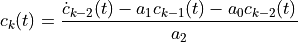
with initial values

$c_0 = \texttt{numpy.array}([c_0^{(0)}, ... , c_0^{(N)}]) \\ c_1 = \texttt{numpy.array}([c_1^{(0)}, ... , c_1^{(N)}])$

with as much computable subsequent coefficients as possible

$c_2 = \texttt{numpy.array}&([c_2^{(0)}, ... , c_2^{(N-1)}]) \\ c_3 = \texttt{numpy.array}&([c_3^{(0)}, ... , c_3^{(N-1)}]) \\ &\vdots \\ c_{2N-1} = \texttt{numpy.array}&([c_{2N-1}^{(0)}]) \\ c_{2N} = \texttt{numpy.array}&([c_{2N}^{(0)}]).$

Only constant parameters $a_2, a_1, a_0 \in \mathbb R$ supported.

Parameters:

c0 (array_like) – $c_0$
c1 (array_like) – $c_1$
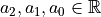
param (array_like) – (a_2, a_1, a_0, None, None)

Returns:

$C = \{0: c_0, 1: c_1, ..., 2N-1: c_{2N-1}, 2N: c_{2N}\}$

Return type:

dict

gevrey_tanh(T, n, sigma=1.1, K=2, length_t=None)¶

Provide Gevrey function

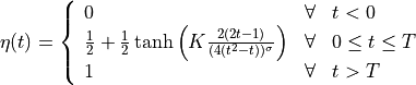
$\eta(t) = \left\{ \begin{array}{lcl} 0 & \forall & t<0 \\ \frac{1}{2} + \frac{1}{2}\tanh \left(K \frac{2(2t-1)} {(4(t^2-t))^\sigma} \right) & \forall & 0\le t \le T \\ 1 & \forall & t>T \end{array} \right.$

with the Gevrey-order $\rho=1+\frac{1}{\sigma}$ and the derivatives up to order n.

Note

For details of the recursive calculation of the derivatives see:

Rudolph, J., J. Winkler und F. Woittennek: Flatness Based Control of Distributed Parameter Systems: Examples and Computer Exercises from Various Technological Domains (Berichte aus der Steuerungs- und Regelungstechnik). Shaker Verlag GmbH, Germany, 2003.

Parameters:

T (numbers.Number) – End of the time domain=[0, T].
n (int) – The derivatives will calculated up to order n.
sigma (numbers.Number) – Constant $\sigma$ to adjust the Gevrey order $\rho=1+\frac{1}{\sigma}$ of $\varphi(t)$ .
K (numbers.Number) – Constant to adjust the slope of $\varphi(t)$ .
length_t (int) – Ammount of sample points to use. Default: int(50 * T)

Returns:

numpy.array([[ $\varphi(t)$ ], … , [ $\varphi^{(n)}(t)$ ]])
t: numpy.array([0,…,T])

Return type:

tuple

power_series(z, t, C, spatial_der_order=0, temporal_der_order=0)¶

Compute the function values

$x^{(j,i)}(z,t)=\sum_{k=0}^{N} c_{k+j}^{(i)}(t) \frac{z^k}{k!}.$

Parameters:

z (array_like) – Spatial steps to compute.
t (array like) – Temporal steps to compute.
C (dict) –
Coeffient dictionary which keys correspond to the coefficient index. The values are 2D numpy.array’s. For example C[1] should provide a 2d-array with the coefficient $c_1(t)$ and at least $i$ temporal derivatives

$\text{np.array}([c_1^{(0)}(t), ... , c_1^{(i)}(t)]).$
spatial_der_order (int) – Spatial derivative order $j$ .
temporal_der_order (int) – Temporal derivative order $i$ .

Returns:

Array of shape (len(t), len(z)).

Return type:

numpy.array

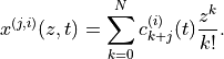
temporal_derived_power_series(z, C, up_to_order, series_termination_index, spatial_der_order=0)¶

Compute the temporal derivatives

$q^{(j,i)}(z=z^*,t) = \sum_{k=0}^{N} \underbrace{c_{k+j}^{(i)}}_{\text{C[k+j][i,:]}} \frac{{z^*}^k}{k!}, \qquad i=0,...,n.$

Parameters:

z (numbers.Number) – Evaluation point $z^*$ .
C (dict) –
Coefficient dictionary whose keys correspond to the coefficient index. The values are 2D numpy.arrays. For example C[1] should provide a 2d-array with the coefficient $c_1(t)$ and at least $n$ temporal derivatives

$\text{np.array}([c_1^{(0)}(t), ... , c_1^{(i)}(t)]) .$
up_to_order (int) – Maximum temporal derivative order $n$ to compute.
series_termination_index (int) – Series termination index $N$ .
spatial_der_order (int) – Spatial derivative order $j$ .

Returns: