Simulation¶

PDE Simulation Basics¶

Write something interesting here :-)

Multiple PDE Simulation¶

The aim of the class CanonicalEquation is to handle more than one pde. For one pde CanonicalForm would be sufficient. The simplest way to get the required $N$ CanonicalEquation’s is to define your problem in $N$ WeakFormulation’s and make use of parse_weak_formulations(). The thus obtained $N$ CanonicalEquation’s you can pass to create_state_space to derive a state space representation of your multi pde system.

Each CanonicalEquation object hold one dominant CanonicalForm and at maximum $N-1$ other CanonicalForm’s.

$\begin{align*} 1\text{st CanonicalForms object} \\ \left. E_{1,n_1} \boldsymbol x_1^{*(n_1)}(t) + \cdots + E_{1,0}\boldsymbol x_1^{*(0)}(t) + \boldsymbol f_1 + G_1 \boldsymbol u(t) = 0 \right\}&\text{dynamic CanonicalForm} \\ \left.\begin{array}{rl} H_{1:2,n_2-1} \boldsymbol x_2^{*(n_2-1)}(t) + \cdots + H_{1:2,0}\boldsymbol x_2^{*(0)}(t) & = 0 \\ & \vdots \\ H_{1:N,n_N-1} \boldsymbol x_N^{*(n_N-1)}(t) + \cdots + H_{1:N,0}\boldsymbol x_N^{*(0)}(t) & = 0 \\ \end{array}\right\}&\text{N-1 static CanonicalForm's} \\ \vdots \hphantom{dddddddddddd} \\ \vdots \hphantom{dddddddddddd} \\ \vdots \hphantom{dddddddddddd} \\ N\text{th CanonicalForms object} \\ \left. E_{N,n_N} \boldsymbol x_N^{*(n_N)}(t) + \cdots + E_{N,0}\boldsymbol x_N^{*(0)}(t) + \boldsymbol f_N + G_N \boldsymbol u(t) = 0 \right\}&\text{dynamic CanonicalForm} \\ \left.\begin{array}{rl} H_{N:1,n_1-1} \boldsymbol x_1^{*(n_1-1)}(t) + \cdots + H_{N:1,0}\boldsymbol x_1^{*(0)}(t) & = 0 \\ & \vdots \\ H_{N:N-1,n_{N-1}-1} \boldsymbol x_{N-1}^{*(n_{N-1}-1)}(t) + \cdots + H_{N:N-1,0}\boldsymbol x_N^{*(0)}(t) & = 0 \\ \end{array}\right\}&\text{N-1 static CanonicalForm's} \\ \end{align*}$

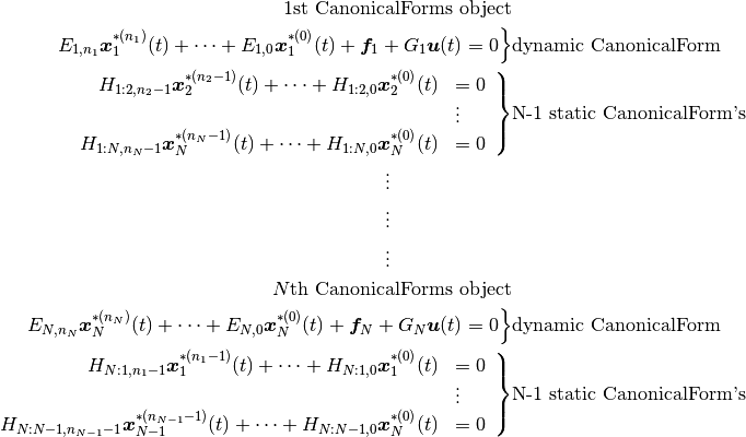
They are interpreted as

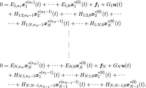
$\begin{align*} 0 &= E_{1,n_1} \boldsymbol x_1^{*(n_1)}(t) + \cdots + E_{1,0}\boldsymbol x_1^{*(0)}(t) + \boldsymbol f_1 + G_1 \boldsymbol u(t) \\ &\hphantom = + H_{1:2,n_2-1} \boldsymbol x_2^{*(n_2-1)}(t) + \cdots + H_{1:2,0}\boldsymbol x_2^{*(0)}(t) + \cdots \\ &\hphantom = \cdots + H_{1:N,n_N-1} \boldsymbol x_N^{*(n_N-1)}(t) + \cdots + H_{1:N,0}\boldsymbol x_N^{*(0)}(t) \\ & \hphantom{ddddddddddddddddddddddd}\vdots \\ & \hphantom{ddddddddddddddddddddddd}\vdots \\ & \hphantom{ddddddddddddddddddddddd}\vdots \\ 0 &= E_{N,n_N} \boldsymbol x_N^{*(n_N)}(t) + \cdots + E_{N,0}\boldsymbol x_N^{*(0)}(t) + \boldsymbol f_N + G_N \boldsymbol u(t) \\ &\hphantom = + H_{N:1,n_1-1} \boldsymbol x_1^{*(n_1-1)}(t) + \cdots + H_{N:1,0}\boldsymbol x_1^{*(0)}(t) + \cdots \\ &\hphantom = \cdots + H_{N:N-1,n_{N-1}-1} \boldsymbol x_{N-1}^{*(n_{N-1}-1)}(t) + \cdots + H_{N:N-1,0}\boldsymbol x_{N-1}^{*(0)}(t). \end{align*}$

These $N$ equations can simply expressed in a state space model

$\dot{\boldsymbol{x}}^*(t) = A\boldsymbol{x}*(t) + B\boldsymbol{u}(t) + \boldsymbol f$

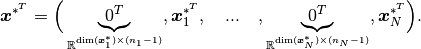
with the weights vector

$\boldsymbol x^{*^T} = \Big(\underbrace{0^T}_{\mathbb{R}^{\text{dim}(\boldsymbol x_1^*)\times (n_1-1)}}, \boldsymbol x_1^{*^T}, \quad ... \quad, \underbrace{0^T}_{\mathbb{R}^{\text{dim}(\boldsymbol x_{N}^*) \times (n_{N}-1)}}, \boldsymbol x_{N}^{*^T}\Big).$