Simulation
Simulation infrastructure with helpers and data structures for preprocessing of the given equations and functions for postprocessing of simulation data.
-
class
CanonicalEquation(name, dominant_lbl=None)[source]¶ Bases:
objectWrapper object, holding several entities of canonical forms for different weight-sets that form an equation when summed up. After instantiation, this object can be filled with information by passing the corresponding coefficients to
add_to(). When the parsing process is completed and all coefficients have been collected, callingfinalize()is required to compute all necessary information for further processing. When finalized, this object provides access to the dominant form of this equation.- Parameters
name (str) – Unique identifier of this equation.
dominant_lbl (str) – Label of the variable that dominates this equation.
-
add_to(self, weight_label, term, val, column=None)[source]¶ Add the provided val to the canonical form for weight_label, see
CanonicalForm.add_to()for further information.
-
dominant_form(self)¶ direct access to the dominant
CanonicalForm.Note
finalize()must be called first.- Returns
the dominant canonical form
- Return type
-
finalize(self)[source]¶ Finalize the Object. After the complete formulation has been parsed and all terms have been sorted into this Object via
add_to()this function has to be called to inform this object about it. Furthermore, the f and G parts of the static_form will be copied to the dominant form for easier state-space transformation.Note
This function must be called to use the
dominant_formattribute.
-
finalize_dynamic_forms(self)[source]¶ Finalize all dynamic forms. See method
CanonicalForm.finalize().
-
input_function(self)¶ The input handles for the equation.
-
static_form(self)¶ WeakFormthat does not depend on any weights. :return:
-
class
CanonicalForm(name=None)[source]¶ Bases:
objectThe canonical form of an nth order ordinary differential equation system.
-
add_to(self, term, value, column=None)[source]¶ Adds the value
valueto termterm.termis a dict that describes which coefficient matrix of the canonical form the value shall be added to.- Parameters
term (dict) –
Targeted term in the canonical form h. It has to contain:
name: Type of the coefficient matrix: ‘E’, ‘f’, or ‘G’.
order: Temporal derivative order of the assigned weights.
exponent: Exponent of the assigned weights.
value (
numpy.ndarray) – Value to add.column (int) – Add the value only to one column of term (useful if only one dimension of term is known).
-
convert_to_state_space(self)[source]¶ Convert the canonical ode system of order n a into an ode system of order 1.
Note
This will only work if the highest derivative order of the given form can be isolated. This is the case if the highest order is only present in one power and the equation system can therefore be solved for it.
- Returns
- Return type
StateSpaceobject
-
finalize(self)[source]¶ Finalizes the object. This method must be called after all terms have been added by
add_to()and beforeconvert_to_state_space()can be called. This functions makes sure that the formulation can be converted into state space form (highest time derivative only comes in one power) and collects information like highest derivative order, it’s power and the sizes of current and state-space state vector (dim_x resp. dim_xb). Furthermore, the coefficient matrix of the highest derivative order e_n_pb and it’s inverse are made accessible.
-
get_terms(self)[source]¶ Return all coefficient matrices of the canonical formulation.
- Returns
Structure: Type > Order > Exponent.
- Return type
Cascade of dictionaries
-
input_function(self)
-
-
class
Domain(bounds=None, num=None, step=None, points=None)[source]¶ Bases:
objectHelper class that manages ranges for data evaluation, containing parameters.
- Parameters
bounds (tuple) – Interval bounds.
num (int) – Number of points in interval.
step (numbers.Number) – Distance between points (if homogeneous).
points (array_like) – Points themselves.
Note
If num and step are given, num will take precedence.
-
bounds(self)
-
ndim(self)
-
points(self)
-
step(self)
-
class
EmptyInput(dim)[source]¶ Bases:
pyinduct.simulation.SimulationInputBase class for all objects that want to act as an input for the time-step simulation.
The calculated values for each time-step are stored in internal memory and can be accessed by
get_results()(after the simulation is finished).Note
Due to the underlying solver, this handle may get called with time arguments, that lie outside of the specified integration domain. This should not be a problem for a feedback controller but might cause problems for a feedforward or trajectory implementation.
-
class
EquationTerm(scale, arg)[source]¶ Bases:
objectBase class for all accepted terms in a weak formulation.
- Parameters
scale –
arg –
-
class
EvalData(input_data, output_data, input_labels=None, input_units=None, enable_extrapolation=False, fill_axes=False, fill_value=None, name=None)[source]¶ This class helps managing any kind of result data.
The data gained by evaluation of a function is stored together with the corresponding points of its evaluation. This way all data needed for plotting or other postprocessing is stored in one place. Next to the points of the evaluation the names and units of the included axes can be stored. After initialization an interpolator is set up, so that one can interpolate in the result data by using the overloaded
__call__()method.- Parameters
input_data – (List of) array(s) holding the axes of a regular grid on which the evaluation took place.
output_data – The result of the evaluation.
- Keyword Arguments
input_labels – (List of) labels for the input axes.
input_units – (List of) units for the input axes.
name – Name of the generated data set.
fill_axes – If the dimension of output_data is higher than the length of the given input_data list, dummy entries will be appended until the required dimension is reached.
enable_extrapolation (bool) – If True, internal interpolators will allow extrapolation. Otherwise, the last giben value will be repeated for 1D cases and the result will be padded with zeros for cases > 1D.
fill_value – If invalid data is encountered, it will be replaced with this value before interpolation is performed.
Examples
When instantiating 1d EvalData objects, the list can be omitted
>>> axis = Domain((0, 10), 5)
>>> data = np.random.rand(5,)
>>> e_1d = EvalData(axis, data)
For other cases, input_data has to be a list
>>> axis1 = Domain((0, 0.5), 5)
>>> axis2 = Domain((0, 1), 11)
>>> data = np.random.rand(5, 11)
>>> e_2d = EvalData([axis1, axis2], data)
Adding two Instances (if the boundaries fit, the data will be interpolated on the more coarse grid.) Same goes for subtraction and multiplication.
>>> e_1 = EvalData(Domain((0, 10), 5), np.random.rand(5,))
>>> e_2 = EvalData(Domain((0, 10), 10), 100*np.random.rand(5,))
>>> e_3 = e_1 + e_2
>>> e_3.output_data.shape
(5,)
Interpolate in the output data by calling the object
>>> e_4 = EvalData(np.array(range(5)), 2*np.array(range(5))))
>>> e_4.output_data
array([0, 2, 4, 6, 8])
>>> e_5 = e_4([2, 5])
>>> e_5.output_data
array([4, 8])
>>> e_5.output_data.size
2
one may also give a slice
>>> e_6 = e_4(slice(1, 5, 2))
>>> e_6.output_data
array([2., 6.])
>>> e_5.output_data.size
2
For multi-dimensional interpolation a list has to be provided
>>> e_7 = e_2d([[.1, .5], [.3, .4, .7)])
>>> e_7.output_data.shape
(2, 3)
-
abs(self)[source]¶ Get the absolute value of the elements form self.output_data .
- Returns
EvalDatawith self.input_data and output_data as result of absolute value calculation.
-
add(self, other, from_left=True)[source]¶ Perform the element-wise addition of the output_data arrays from self and other
This method is used to support addition by implementing __add__ (fromLeft=True) and __radd__(fromLeft=False)). If other** is a
EvalData, the input_data lists of self and other are adjusted usingadjust_input_vectors()The summation operation is performed on the interpolated output_data. If other is anumbers.Numberit is added according to numpy’s broadcasting rules.
-
adjust_input_vectors(self, other)[source]¶ Check the the inputs vectors of self and other for compatibility (equivalence) and harmonize them if they are compatible.
The compatibility check is performed for every input_vector in particular and examines whether they share the same boundaries. and equalize to the minimal discretized axis. If the amount of discretization steps between the two instances differs, the more precise discretization is interpolated down onto the less precise one.
- Parameters
other (
EvalData) – Other EvalData class.- Returns
(list) - New common input vectors.
(numpy.ndarray) - Interpolated self output_data array.
(numpy.ndarray) - Interpolated other output_data array.
- Return type
tuple
-
interpolate(self, interp_axis)[source]¶ Main interpolation method for output_data.
If one of the output dimensions is to be interpolated at one single point, the dimension of the output will decrease by one.
- Parameters
interp_axis (list(list)) – axis positions in the form
1D (-) – axis with axis=[1,2,3]
2D (-) – [axis1, axis2] with axis1=[1,2,3] and axis2=[0,1,2,3,4]
- Returns
EvalDatawith interp_axis as new input_data and interpolated output_data.
-
matmul(self, other, from_left=True)[source]¶ Perform the matrix multiplication of the output_data arrays from self and other .
This method is used to support matrix multiplication (@) by implementing __matmul__ (from_left=True) and __rmatmul__(from_left=False)). If other** is a
EvalData, the input_data lists of self and other are adjusted usingadjust_input_vectors(). The matrix multiplication operation is performed on the interpolated output_data. If other is anumbers.Numberit is handled according to numpy’s broadcasting rules.
-
mul(self, other, from_left=True)[source]¶ Perform the element-wise multiplication of the output_data arrays from self and other .
This method is used to support multiplication by implementing __mul__ (from_left=True) and __rmul__(from_left=False)). If other** is a
EvalData, the input_data lists of self and other are adjusted usingadjust_input_vectors(). The multiplication operation is performed on the interpolated output_data. If other is anumbers.Numberit is handled according to numpy’s broadcasting rules.
-
sqrt(self)[source]¶ Radicate the elements form self.output_data element-wise.
- Returns
EvalDatawith self.input_data and output_data as result of root calculation.
-
sub(self, other, from_left=True)[source]¶ Perform the element-wise subtraction of the output_data arrays from self and other .
This method is used to support subtraction by implementing __sub__ (from_left=True) and __rsub__(from_left=False)). If other** is a
EvalData, the input_data lists of self and other are adjusted usingadjust_input_vectors(). The subtraction operation is performed on the interpolated output_data. If other is anumbers.Numberit is handled according to numpy’s broadcasting rules.
-
class
FieldVariable(function_label, order=0, 0, weight_label=None, location=None, exponent=1, raised_spatially=False)[source]¶ Bases:
pyinduct.placeholder.PlaceholderClass that represents terms of the systems field variable
 .
.- Parameters
function_label (str) – Label of shapefunctions to use for approximation, see
register_base()for more information about how to register an approximation basis.tuple of int (order) – Tuple of temporal_order and spatial_order derivation order.
weight_label (str) – Label of weights for which coefficients are to be calculated (defaults to function_label).
location – Where the expression is to be evaluated.
exponent – Exponent of the term.
Examples
Assuming some shapefunctions have been registered under the label
"phi"the following expressions hold:>>> x_dt_dzz = FieldVariable("phi", order=(1, 2))
>>> x_dtt_at_3 = FieldVariable("phi", order=(2, 0), location=3)
-
derive(self, *, temp_order=0, spat_order=0)[source]¶ Derive the expression to the specified order.
- Parameters
temp_order – Temporal derivative order.
spat_order – Spatial derivative order.
- Returns
The derived expression.
- Return type
Note
This method uses keyword only arguments, which means that a call will fail if the arguments are passed by order.


-
class
Function(eval_handle, domain=- np.inf, np.inf, nonzero=- np.inf, np.inf, derivative_handles=None)[source]¶ Bases:
pyinduct.core.BaseFractionMost common instance of a
BaseFraction. This class handles all tasks concerning derivation and evaluation of functions. It is used broad across the toolbox and therefore incorporates some very specific attributes. For example, to ensure the accurateness of numerical handling functions may only evaluated in areas where they provide nonzero return values. Also their domain has to be taken into account. Therefore the attributes domain and nonzero are provided.To save implementation time, ready to go version like
LagrangeFirstOrderare provided in thepyinduct.simulationmodule.For the implementation of new shape functions subclass this implementation or directly provide a callable eval_handle and callable derivative_handles if spatial derivatives are required for the application.
- Parameters
eval_handle (callable) – Callable object that can be evaluated.
domain ((list of) tuples) – Domain on which the eval_handle is defined.
nonzero (tuple) – Region in which the eval_handle will return
output. Must be a subset of domain (nonzero) –
derivative_handles (list) – List of callable(s) that contain
of eval_handle (derivatives) –
-
add_neutral_element(self)[source]¶ Return the neutral element of addition for this object.
In other words: self + ret_val == self.
-
derivative_handles(self)
-
derive(self, order=1)[source]¶ Spatially derive this
Function.This is done by neglecting order derivative handles and to select handle
 as the new evaluation_handle.
- Parameters
order (int) – the amount of derivations to perform
- Raises
TypeError – If order is not of type int.
ValueError – If the requested derivative order is higher than the provided one.
- Returns
Functionthe derived function.
-
static
from_data(x, y, **kwargs)[source]¶ Create a
Functionbased on discrete data by interpolating.The interpolation is done by using
interp1dfrom scipy, the kwargs will be passed.
-
function_handle(self)
-
function_space_hint(self)[source]¶ Return the hint that this function is an element of the an scalar product space which is uniquely defined by the scalar product
scalar_product_hint().Note
If you are working on different function spaces, you have to overwrite this hint in order to provide more properties which characterize your specific function space. For example the domain of the functions.
-
get_member(self, idx)[source]¶ Implementation of the abstract parent method.
Since the
Functionhas only one member (itself) the parameter idx is ignored and self is returned.- Parameters
idx – ignored.
- Returns
self
-
mul_neutral_element(self)[source]¶ Return the neutral element of multiplication for this object.
In other words: self * ret_val == self.
-
raise_to(self, power)[source]¶ Raises the function to the given power.
Warning
Derivatives are lost after this action is performed.
- Parameters
power (
numbers.Number) – power to raise the function to- Returns
raised function
-
class
Input(function_handle, index=0, order=0, exponent=1)[source]¶ Bases:
pyinduct.placeholder.PlaceholderClass that works as a placeholder for an input of the system.
- Parameters
function_handle (callable) – Handle that will be called by the simulation unit.
index (int) – If the system’s input is vectorial, specify the element to be used.
order (int) – temporal derivative order of this term (See
Placeholder).exponent (numbers.Number) – See
FieldVariable.
Note
if order is nonzero, the callable is expected to return the temporal derivatives of the input signal by returning an array of
len(order)+1.
-
class
IntegralTerm(integrand, limits, scale=1.0)[source]¶ Bases:
pyinduct.placeholder.EquationTermClass that represents an integral term in a weak equation.
- Parameters
integrand –
limits (tuple) –
scale –
-
class
ObserverGain(observer_feedback)[source]¶ Bases:
pyinduct.placeholder.PlaceholderClass that works as a placeholder for the observer error gain.
- Parameters
observer_feedback (
ObserverFeedback) – Handle that will be called by the simulation unit.
-
class
Parameters(**kwargs)[source]¶ Handy class to collect system parameters. This class can be instantiated with a dict, whose keys will the become attributes of the object. (Bunch approach)
- Parameters
kwargs – parameters
-
class
ScalarProductTerm(arg1, arg2, scale=1.0)[source]¶ Bases:
pyinduct.placeholder.EquationTermClass that represents a scalar product in a weak equation.
- Parameters
arg1 – Fieldvariable (Shapefunctions) to be projected.
arg2 – Testfunctions to project on.
scale (Number) – Scaling of expression.
-
class
ScalarTerm(argument, scale=1.0)[source]¶ Bases:
pyinduct.placeholder.EquationTermClass that represents a scalar term in a weak equation.
- Parameters
argument –
scale –
-
class
Scalars(values, target_term=None, target_form=None, test_func_lbl=None)[source]¶ Bases:
pyinduct.placeholder.PlaceholderPlaceholder for scalar values that scale the equation system, gained by the projection of the pde onto the test basis.
Note
The arguments target_term and target_form are used inside the parser. For frontend use, just specify the values.
- Parameters
values – Iterable object containing the scalars for every k-th equation.
target_term – Coefficient matrix to
add_to().target_form – Desired weight set.
-
class
SimulationInput(name='')[source]¶ Bases:
objectBase class for all objects that want to act as an input for the time-step simulation.
The calculated values for each time-step are stored in internal memory and can be accessed by
get_results()(after the simulation is finished).Note
Due to the underlying solver, this handle may get called with time arguments, that lie outside of the specified integration domain. This should not be a problem for a feedback controller but might cause problems for a feedforward or trajectory implementation.
-
clear_cache(self)[source]¶ Clear the internal value storage.
When the same SimulationInput is used to perform various simulations, there is no possibility to distinguish between the different runs when
get_results()gets called. Therefore this method can be used to clear the cache.
-
get_results(self, time_steps, result_key='output', interpolation='nearest', as_eval_data=False)[source]¶ Return results from internal storage for given time steps.
- Raises
Error – If calling this method before a simulation was run.
- Parameters
time_steps – Time points where values are demanded.
result_key – Type of values to be returned.
interpolation – Interpolation method to use if demanded time-steps are not covered by the storage, see
scipy.interpolate.interp1d()for all possibilities.as_eval_data (bool) – Return results as
EvalDataobject for straightforward display.
- Returns
Corresponding function values to the given time steps.
-
-
class
SimulationInputSum(inputs)[source]¶ Bases:
pyinduct.simulation.SimulationInputHelper that represents a signal mixer.
-
class
SimulationInputVector(input_vector)[source]¶ Bases:
pyinduct.simulation.SimulationInputA simulation input which combines
SimulationInputobjects into a column vector.- Parameters
input_vector (array_like) – Simulation inputs to stack.
-
class
StackedBase(base_info)[source]¶ Bases:
pyinduct.core.ApproximationBasisImplementation of a basis vector that is obtained by stacking different bases onto each other. This typically occurs when the bases of coupled systems are joined to create a unified system.
- Parameters
base_info (OrderedDict) –
Dictionary with base_label as keys and dictionaries holding information about the bases as values. In detail, these Information must contain:
sys_name (str): Name of the system the base is associated with.
- order (int): Highest temporal derivative order with which the
base shall be represented in the stacked base.
base (
ApproximationBase): The actual basis.
-
function_space_hint(self)[source]¶ Hint that returns properties that characterize the functional space of the fractions. It can be used to determine if function spaces match.
Note
Overwrite to implement custom functionality.
-
is_compatible_to(self, other)[source]¶ Helper functions that checks compatibility between two approximation bases.
In this case compatibility is given if the two bases live in the same function space.
- Parameters
other (
Approximation Base) – Approximation basis to compare with.
Returns: True if bases match, False if they do not.
-
scalar_product_hint(self)[source]¶ Hint that returns steps for scalar product calculation with elements of this base.
Note
Overwrite to implement custom functionality.
-
transformation_hint(self, info)[source]¶ If info.src_lbl is a member, just return it, using to correct derivative transformation, otherwise return None
- Parameters
info (
TransformationInfo) – Information about the requested transformation.- Returns
transformation handle
-
class
StateSpace(a_matrices, b_matrices, base_lbl=None, input_handle=None, c_matrix=None, d_matrix=None, obs_fb_handle=None)[source]¶ Bases:
objectWrapper class that represents the state space form of a dynamic system where
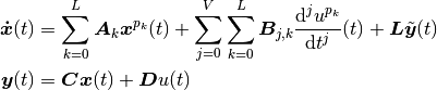
which has been approximated by projection on a base given by weight_label.
- Parameters
a_matrices (dict) – State transition matrices
 for the corresponding powers of
 .
.b_matrices (dict) – Cascaded dictionary for the input matrices
 in the sequence: temporal derivative
order, exponent.
in the sequence: temporal derivative
order, exponent.input_handle (
SimulationInput) – System input .
.c_matrix –

d_matrix –


-
class
TestFunction(function_label, order=0, location=None, approx_label=None)[source]¶ Bases:
pyinduct.placeholder.SpatialPlaceholderClass that works as a placeholder for test functions in an equation.
- Parameters
function_label (str) – Label of the function test base.
order (int) – Spatial derivative order.
location (Number) – Point of evaluation / argument of the function.
approx_label (str) – Label of the approximation test base.
-
class
WeakFormulation(terms, name, dominant_lbl=None)[source]¶ Bases:
objectThis class represents the weak formulation of a spatial problem. It can be initialized with several terms (see children of
EquationTerm). The equation is interpreted as
- Parameters
terms (list) – List of object(s) of type EquationTerm.
name (string) – Name of this weak form.
dominant_lbl (string) – Name of the variable that dominates this weak form.
-
calculate_scalar_product_matrix(base_a, base_b, scalar_product=None, optimize=True)[source]¶ Calculates a matrix
 , whose elements are the scalar products of
each element from base_a and base_b, so that
, whose elements are the scalar products of
each element from base_a and base_b, so that
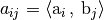 .
.- Parameters
base_a (
ApproximationBase) – Basis abase_b (
ApproximationBase) – Basis bscalar_product – (List of) function objects that are passed the members of the given bases as pairs. Defaults to the scalar product given by base_a
optimize (bool) – Switch to turn on the symmetry based speed up. For development purposes only.
- Returns
matrix
- Return type
numpy.ndarray
-
create_state_space(canonical_equations)[source]¶ Create a state-space system constituted by several
CanonicalEquations(created byparse_weak_formulation())- Parameters
canonical_equations – List of
CanonicalEquation’s.- Raises
ValueError – If compatibility criteria cannot be fulfilled
- Returns
State-space representation of the approximated system
- Return type
-
domain_intersection(first, second)[source]¶ Calculate intersection(s) of two domains.
- Parameters
first (set) – (Set of) tuples defining the first domain.
second (set) – (Set of) tuples defining the second domain.
- Returns
Intersection given by (start, end) tuples.
- Return type
set
-
evaluate_approximation(base_label, weights, temp_domain, spat_domain, spat_order=0, name='')[source]¶ Evaluate an approximation given by weights and functions at the points given in spatial and temporal steps.
- Parameters
weights – 2d np.ndarray where axis 1 is the weight index and axis 0 the temporal index.
base_label (str) – Functions to use for back-projection.
temp_domain (
Domain) – For steps to evaluate at.spat_domain (
Domain) – For points to evaluate at (or in).spat_order – Spatial derivative order to use.
name – Name to use.
- Returns
-
get_base(label)[source]¶ Retrieve registered set of initial functions by their label.
- Parameters
label (str) – String, label of functions to retrieve.
- Returns
initial_functions
-
get_common_form(placeholders)[source]¶ Extracts the common target form from a list of scalars while making sure that the given targets are equivalent.
- Parameters
placeholders – Placeholders with possibly differing target forms.
- Returns
Common target form.
- Return type
str
-
get_common_target(scalars)[source]¶ Extracts the common target from list of scalars while making sure that targets are equivalent.
- Parameters
scalars (
Scalars) –- Returns
Common target.
- Return type
dict
-
get_sim_result(weight_lbl, q, temp_domain, spat_domain, temp_order, spat_order, name='')[source]¶ Create handles and evaluate at given points.
- Parameters
weight_lbl (str) – Label of Basis for reconstruction.
temp_order – Order or temporal derivatives to evaluate additionally.
spat_order – Order or spatial derivatives to evaluate additionally.
q – weights
spat_domain (
Domain) – Domain object providing values for spatial evaluation.temp_domain (
Domain) – Time steps on which rows of q are given.name (str) – Name of the WeakForm, used to generate the data set.
-
get_sim_results(temp_domain, spat_domains, weights, state_space, names=None, derivative_orders=None)[source]¶ Convenience wrapper for
get_sim_result().- Parameters
temp_domain (
Domain) – Time domainspat_domains (dict) – Spatial domain from all subsystems which belongs to state_space as values and name of the systems as keys.
weights (numpy.array) – Weights gained through simulation. For example with
simulate_state_space().state_space (
StateSpace) – Simulated state space instance.names – List of names of the desired systems. If not given all available subssystems will be processed.
derivative_orders (dict) – Desired derivative orders.
- Returns
List of
EvalDataobjects.
-
get_transformation_info(source_label, destination_label, source_order=0, destination_order=0)[source]¶ Provide the weights transformation from one/source base to another/destination base.
- Parameters
source_label (str) – Label from the source base.
destination_label (str) – Label from the destination base.
source_order – Order from the available time derivative of the source weights.
destination_order – Order from the desired time derivative of the destination weights.
- Returns
Transformation info object.
- Return type
-
get_weight_transformation(info)[source]¶ Create a handle that will transform weights from info.src_base into weights for info-dst_base while paying respect to the given derivative orders.
This is accomplished by recursively iterating through source and destination bases and evaluating their
transformation_hints.- Parameters
info (
TransformationInfo) – information about the requested transformation.- Returns
transformation function handle
- Return type
callable
-
integrate_function(func, interval)[source]¶ Numerically integrate a function on a given interval using
complex_quadrature().- Parameters
func (callable) – Function to integrate.
interval (list of tuples) – List of (start, end) values of the intervals to integrate on.
- Returns
(Result of the Integration, errors that occurred during the integration).
- Return type
tuple
-
parse_weak_formulation(weak_form, finalize=False, is_observer=False)[source]¶ Parses a
WeakFormulationthat has been derived by projecting a partial differential equation an a set of test-functions. Within this process, the separating approximation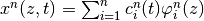 is plugged into
the equation and the separated spatial terms are evaluated, leading to a
ordinary equation system for the weights
is plugged into
the equation and the separated spatial terms are evaluated, leading to a
ordinary equation system for the weights  .
.- Parameters
weak_form – Weak formulation of the pde.
finalize (bool) – Default: False. If you have already defined the dominant labels of the weak formulations you can set this to True. See
CanonicalEquation.finalize()
- Returns
The spatially approximated equation in a canonical form.
- Return type
-
parse_weak_formulations(weak_forms)[source]¶ Convenience wrapper for
parse_weak_formulation().- Parameters
weak_forms – List of
WeakFormulation’s.- Returns
List of
CanonicalEquation’s.
-
project_on_bases(states, canonical_equations)[source]¶ Convenience wrapper for
project_on_base(). Calculate the state, assuming it will be constituted by the dominant base of the respective system. The keys from the dictionaries canonical_equations and states must be the same.- Parameters
states – Dictionary with a list of functions as values.
canonical_equations – List of
CanonicalEquationinstances.
- Returns
Finite dimensional state as 1d-array corresponding to the concatenated dominant bases from canonical_equations.
- Return type
numpy.array
-
register_base(label, base, overwrite=False)[source]¶ Register a basis to make it accessible all over the
pyinductframework.- Parameters
base (
ApproximationBase) – base to registerlabel (str) – String that will be used as label.
overwrite – Force overwrite if a basis is already registered under this label.
-
sanitize_input(input_object, allowed_type)[source]¶ Sanitizes input data by testing if input_object is an array of type allowed_type.
- Parameters
input_object – Object which is to be checked.
allowed_type – desired type
- Returns
input_object
-
set_dominant_labels(canonical_equations, finalize=True)[source]¶ Set the dominant label (dominant_lbl) member of all given canonical equations and check if the problem formulation is valid (see background section: http://pyinduct.readthedocs.io/en/latest/).
If the dominant label of one or more
CanonicalEquationis already defined, the function raise a UserWarning if the (pre)defined dominant label(s) are not valid.- Parameters
canonical_equations – List of
CanonicalEquationinstances.finalize (bool) – Finalize the equations? Default: True.
-
simulate_state_space(state_space, initial_state, temp_domain, settings=None)[source]¶ Wrapper to simulate a system given in state space form:

- Parameters
state_space (
StateSpace) – State space formulation of the system.initial_state – Initial state vector of the system.
temp_domain (
Domain) – Temporal domain object.settings (dict) – Parameters to pass to the
set_integrator()method of thescipy.odeclass, with the integrator name included under the keyname.
- Returns
Time
Domainobject and weights matrix.- Return type
tuple
-
simulate_system(weak_form, initial_states, temporal_domain, spatial_domain, derivative_orders=0, 0, settings=None)[source]¶ Convenience wrapper for
simulate_systems().- Parameters
weak_form (
WeakFormulation) – Weak formulation of the system to simulate.initial_states (numpy.ndarray) – Array of core.Functions for
 .
.temporal_domain (
Domain) – Domain object holding information for time evaluation.spatial_domain (
Domain) – Domain object holding information for spatial evaluation.derivative_orders (tuple) – tuples of derivative orders (time, spat) that shall be evaluated additionally as values
settings – Integrator settings, see
simulate_state_space().
-
simulate_systems(weak_forms, initial_states, temporal_domain, spatial_domains, derivative_orders=None, settings=None, out=list())[source]¶ Convenience wrapper that encapsulates the whole simulation process.
- Parameters
weak_forms ((list of)
WeakFormulation) – (list of) Weak formulation(s) of the system(s) to simulate.initial_states (dict, numpy.ndarray) – Array of core.Functions for
.temporal_domain (
Domain) – Domain object holding information for time evaluation.spatial_domains (dict) – Dict with
Domainobjects holding information for spatial evaluation.derivative_orders (dict) – Dict, containing tuples of derivative orders (time, spat) that shall be evaluated additionally as values
settings – Integrator settings, see
simulate_state_space().out (list) –
List from user namespace, where the following intermediate results will be appended:
canonical equations (list of types:
CanocialEquation)state space object (type:
StateSpace)initial weights (type:
numpy.array)simulation results/weights (type:
numpy.array)
Note
The name attributes of the given weak forms must be unique!
- Returns
List of
EvalDataobjects, holding the results for the FieldVariable and demanded derivatives.- Return type
list
-
vectorize_scalar_product(first, second, scalar_product)[source]¶ Call the given
scalar_productin a loop for the arguments inleftandright.Given two vectors of functions
and

this function computes
 where
where
Herein,
 denotes the complex conjugate and
 as well as
  are derived by computing the
intersection of the nonzero areas of the involved functions.
are derived by computing the
intersection of the nonzero areas of the involved functions.- Parameters
first (callable or
numpy.ndarray) – (1d array of n) callable(s)second (callable or
numpy.ndarray) – (1d array of n) callable(s)
- Raises
ValueError, if the provided arrays are not equally long. –
- Returns
Array of inner products
- Return type
numpy.ndarray