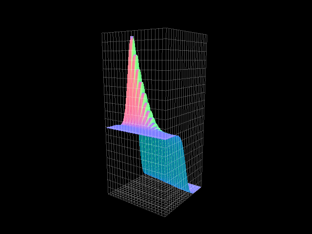
R.a.d. eq. with dirichlet b.c. (fem approximation)¶

Simulation of the reaction-advection-diffusion equation with dirichlet boundary condition by $z=0$ and dirichlet actuation by $z=l$ .

$\begin{align*} \dot{x}(z,t) = a_2x''&(z,t) + a_1x'(z,t) + a_0x(z,t) && z\in (0, l), t>0\\ x(z,0) &= x_0(z) && z\in [0,l]\\ x(0,t) &= 0 && t>0\\ x(l,t) &= u(t) && t>0 \end{align*}$

example: heat equation
- $a_2=1,\quad a_1= 0, \quad a_0=0, \quad x_0(z)=0$
- $u(t)$ –> pyinduct.trajectory.RadTrajectory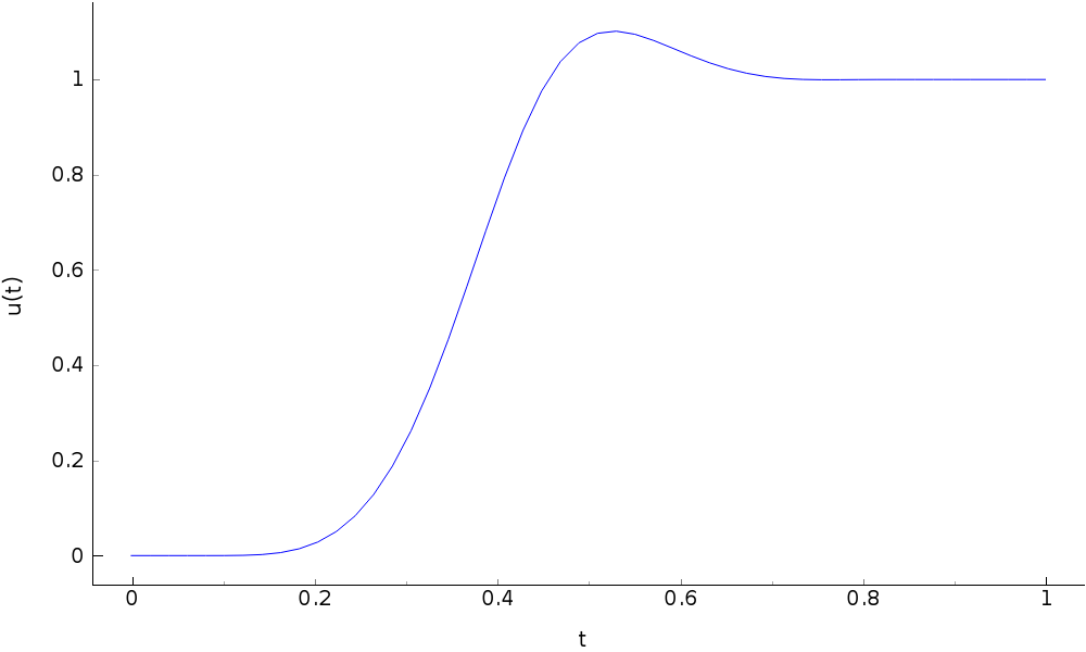
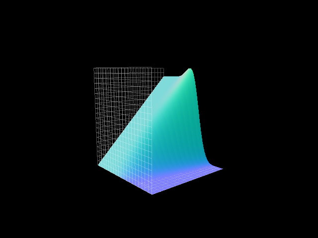
- $x(z,t)$
- $x'(z,t)$
- corresponding 3d plots

$x(z,t)$	$x'(z,t)$

with:
- inital functions $\varphi_1(z),...,\varphi_{n+1}(z)$
- test functions $\varphi_1(z),...,\varphi_n(z)$
- where the functions $\varphi_1(z),..,\varphi_n(z)$ met the homogeneous b.c.
  
  $\varphi_1(l),..,\varphi_n(l)=\varphi_1(0),..,\varphi_n(0)=0$
- only $\varphi_{n+1}$ can draw the actuation
- functions $\varphi_1(z),...,\varphi_{n+1}(z)$ e.g. from type pyinduct.shapefunctions.LagrangeFirstOrder or pyinduct.shapefunctions.LagrangeSecondOrder, see pyinduct.shapefunctions
approach:

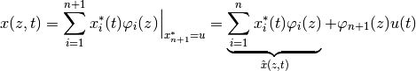
$x(z,t) = \sum_{i=1}^{n+1} x_i^*(t) \varphi_i(z)\Big|_{x^*_{n+1}=u} = \underbrace{\sum_{i=1}^{n} x_i^*(t) \varphi_i(z)}_{\hat x(z,t)} + \varphi_{n+1}(z) u(t)$

weak formulation…

$\begin{align*} \langle\dot{x}(z,t),\varphi_j(z)\rangle &= a_2 \langle x''(z,t),\varphi_j(z)\rangle \\ &\hphantom =+ a_1 \langle x'(z,t), \varphi_j(z)\rangle + a_0 \langle x(z,t), \varphi_j(z)\rangle && j=1,...,n \end{align*}$

… and derivation shift to work with lagrange 1st order initial functions

$\begin{align*} \langle\dot{x}(z,t),\varphi_j(z)\rangle &= \overbrace{[a_2 [x'(z,t)\varphi_j(z)]_0^l}^{=0} - a_2 \langle x'(z,t),\varphi'_j(z)\rangle \\ &\hphantom =+ a_1 \langle x'(z,t), \varphi_j(z)\rangle + a_0 \langle x(z,t), \varphi_j(z)\rangle && j=1,...,n \\ \langle\dot{\hat{x}}(z,t),\varphi_j(z)\rangle + \langle\varphi_{N+1}(z),\varphi_j(z)\rangle \dot u(t) &= - a_2 \langle \hat x'(z,t),\varphi'_j(z)\rangle - a_2 \langle \varphi'_{N+1}(z),\varphi'_j(z)\rangle u(t) \\ &\hphantom =+ a_1 \langle \hat x'(z,t), \varphi_j(z)\rangle + a_1 \langle \varphi'_{N+1}(z), \varphi_j(z)\rangle u(t) + \\ &\hphantom =+ a_0 \langle \hat x(z,t), \varphi_j(z)\rangle + a_0 \langle \varphi_{N+1}(z), \varphi_j(z)\rangle u(t) && j=1,...,n \end{align*}$

leads to state space model for the weights $\boldsymbol{x}^*=(x_1^*,...,x_n^*)^T$ :

$\begin{align*} \dot{\boldsymbol{x}}^*(t) = A \boldsymbol x^*(t) + \boldsymbol b_0 u(t) + \boldsymbol b_1 \dot{u}(t) \end{align*}$

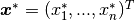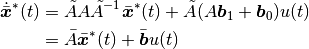
input derivative elimination through the transformation:
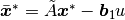
- $\bar{\boldsymbol{x}}^* = \tilde A \boldsymbol x^* - \boldsymbol{b}_1 u$
- $\text{e.g.: } \tilde A = I$
- leads to

$\begin{align*} \dot{\bar{\boldsymbol{x}}}^*(t) &= \tilde A A\tilde A^{-1} \bar{\boldsymbol{x}}^*(t) + \tilde A(A\boldsymbol b_1 + \boldsymbol b_0) u(t) \\ &= \bar A \bar{\boldsymbol{x}}^*(t) +\bar{\boldsymbol{b}} u(t) \end{align*}$

source code:

import numpy as np
import pyinduct as pi
import pyinduct.parabolic as parabolic


def run(show_plots):
    n_fem = 17
    T = 1
    l = 1
    y0 = -1
    y1 = 4

    param = [1, 0, 0, None, None]
    # or try these:
    # param = [1, -0.5, -8, None, None]   #  :)))
    a2, a1, a0, _, _ = param

    temp_domain = pi.Domain(bounds=(0, T), num=100)
    spat_domain = pi.Domain(bounds=(0, l), num=n_fem * 11)

    # initial and test functions
    nodes = pi.Domain(spat_domain.bounds, num=n_fem)
    fem_base = pi.LagrangeFirstOrder.cure_interval(nodes)
    act_fem_base = pi.Base(fem_base[-1])
    not_act_fem_base = pi.Base(fem_base[1:-1])
    vis_fems_base = pi.Base(fem_base)

    pi.register_base("act_base", act_fem_base)
    pi.register_base("sim_base", not_act_fem_base)
    pi.register_base("vis_base", vis_fems_base)

    # trajectory
    u = parabolic.RadFeedForward(l, T,
                                 param_original=param,
                                 bound_cond_type="dirichlet",
                                 actuation_type="dirichlet",
                                 y_start=y0, y_end=y1)

    # weak form
    x = pi.FieldVariable("sim_base")
    x_dt = x.derive(temp_order=1)
    x_dz = x.derive(spat_order=1)
    phi = pi.TestFunction("sim_base")
    phi_dz = phi.derive(1)
    act_phi = pi.ScalarFunction("act_base")
    act_phi_dz = act_phi.derive(1)

    weak_form = pi.WeakFormulation([
        # ... of the homogeneous part of the system
        pi.IntegralTerm(pi.Product(x_dt, phi),
                        limits=spat_domain.bounds),
        pi.IntegralTerm(pi.Product(x_dz, phi_dz),
                        limits=spat_domain.bounds,
                        scale=a2),
        pi.IntegralTerm(pi.Product(x_dz, phi),
                        limits=spat_domain.bounds,
                        scale=-a1),
        pi.IntegralTerm(pi.Product(x, phi),
                        limits=spat_domain.bounds,
                        scale=-a0),

        # ... of the inhomogeneous part of the system
        pi.IntegralTerm(pi.Product(pi.Product(act_phi, phi),
                                   pi.Input(u, order=1)),
                        limits=spat_domain.bounds),
        pi.IntegralTerm(pi.Product(pi.Product(act_phi_dz, phi_dz),
                                   pi.Input(u)),
                        limits=spat_domain.bounds,
                        scale=a2),
        pi.IntegralTerm(pi.Product(pi.Product(act_phi_dz, phi),
                                   pi.Input(u)),
                        limits=spat_domain.bounds,
                        scale=-a1),
        pi.IntegralTerm(pi.Product(pi.Product(act_phi, phi),
                                   pi.Input(u)),
                        limits=spat_domain.bounds,
                        scale=-a0)],
        name="main_system")

    # system matrices \dot x = A x + b0 u + b1 \dot u
    cf = pi.parse_weak_formulation(weak_form)
    ss = pi.create_state_space(cf)

    a_mat = ss.A[1]
    b0 = ss.B[0][1]
    b1 = ss.B[1][1]

    # transformation into \dot \bar x = \bar A \bar x + \bar b u
    a_tilde = np.diag(np.ones(a_mat.shape[0]), 0)
    a_tilde_inv = np.linalg.inv(a_tilde)

    a_bar = (a_tilde @ a_mat) @ a_tilde_inv
    b_bar = a_tilde @ (a_mat @ b1) + b0

    # simulation
    def x0(z):
        return 0 + y0 * z

    start_func = pi.Function(x0, domain=spat_domain.bounds)
    full_start_state = np.array([pi.project_on_base(start_func,
                                               pi.get_base("vis_base")
                                               )]).flatten()
    initial_state = full_start_state[1:-1]

    start_state_bar = a_tilde @ initial_state - (b1 * u(time=0)).flatten()
    ss = pi.StateSpace(a_bar, b_bar, base_lbl="sim", input_handle=u)
    sim_temp_domain, sim_weights_bar = pi.simulate_state_space(ss,
                                                               start_state_bar,
                                                               temp_domain)

    # back-transformation
    u_vec = np.reshape(u.get_results(sim_temp_domain), (len(temp_domain), 1))
    sim_weights = sim_weights_bar @ a_tilde_inv + u_vec @ b1.T

    # visualisation
    plots = list()
    save_pics = False
    vis_weights = np.hstack((np.zeros_like(u_vec), sim_weights, u_vec))

    eval_d = pi.evaluate_approximation("vis_base",
                                       vis_weights,
                                       sim_temp_domain,
                                       spat_domain,
                                       spat_order=0)
    der_eval_d = pi.evaluate_approximation("vis_base",
                                           vis_weights,
                                           sim_temp_domain,
                                           spat_domain,
                                           spat_order=1)

    if show_plots:
        plots.append(pi.PgAnimatedPlot(eval_d,
                                 labels=dict(left='x(z,t)', bottom='z'),
                                 save_pics=save_pics))
        plots.append(pi.PgAnimatedPlot(der_eval_d,
                                 labels=dict(left='x\'(z,t)', bottom='z'),
                                 save_pics=save_pics))

        win1 = pi.surface_plot(eval_d, title="x(z,t)")
        win2 = pi.surface_plot(der_eval_d, title="x'(z,t)")

        # save pics
        if save_pics:
            path = pi.save_2d_pg_plot(u.get_plot(), 'rad_dirichlet_traj')[1]
            win1.gl_widget.grabFrameBuffer().save(path + 'rad_dirichlet_3d_x.png')
            win2.gl_widget.grabFrameBuffer().save(path + 'rad_dirichlet_3d_dx.png')
        pi.show()

    pi.tear_down(("act_base", "sim_base", "vis_base"))


if __name__ == "__main__":
    run(True)