Eigenfunctions
This modules provides eigenfunctions for a certain set of second order spatial operators. Therefore functions for the computation of the corresponding eigenvalues are included. The functions which compute the eigenvalues are deliberately separated from the predefined eigenfunctions in order to handle transformations and reduce effort within the controller implementation.
-
class
AddMulFunction(function)¶ Bases:
object(Temporary) Function class which can multiplied with scalars and added with functions. Only needed to compute the matrix (of scalars) vector (of functions) product in
FiniteTransformFunction. Will be no longer needed whenFunctionis overloaded with__add__and__mul__operator.- Parameters
function (callable) –
-
class
Base(fractions, matching_base_lbls=None, intermediate_base_lbls=None)¶ Bases:
pyinduct.core.ApproximationBasisBase class for approximation bases.
In general, a
Baseis formed by a certain amount ofBaseFractionsand therefore forms finite-dimensional subspace of the distributed problem’s domain. Most of the time, the user does not need to interact with this class.- Parameters
fractions (iterable of
BaseFraction) – List, array or dict ofBaseFraction’smatching_base_lbls (list of str) – List of labels from exactly matching bases, for which no transformation is necessary. Useful for transformations from bases that ‘live’ in different function spaces but evolve with the same time dynamic/coefficients (e.g. modal bases).
intermediate_base_lbls (list of str) – If it is certain that this base instance will be asked (as destination base) to return a transformation to a source base, whose implementation is cumbersome, its label can be provided here. This will trigger the generation of the transformation using build-in features. The algorithm, implemented in
get_weights_transformationis then called again with the intermediate base as destination base and the ‘old’ source base. With this technique arbitrary long transformation chains are possible, if the provided intermediate bases again define intermediate bases.
-
derive(self, order)¶ Basic implementation of derive function. Empty implementation, overwrite to use this functionality.
- Parameters
order (
numbers.Number) – derivative order- Returns
derived object
- Return type
-
function_space_hint(self)¶ Hint that returns properties that characterize the functional space of the fractions. It can be used to determine if function spaces match.
Note
Overwrite to implement custom functionality.
-
get_attribute(self, attr)¶ Retrieve an attribute from the fractions of the base.
- Parameters
attr (str) – Attribute to query the fractions for.
- Returns
Array of
len(fractions)holding the attributes. With None entries if the attribute is missing.- Return type
np.ndarray
-
raise_to(self, power)¶ Factory method to obtain instances of this base, raised by the given power.
- Parameters
power – power to raise the basis onto.
-
scalar_product_hint(self)¶ Hint that returns steps for scalar product calculation with elements of this base.
Note
Overwrite to implement custom functionality.
-
scale(self, factor)¶ Factory method to obtain instances of this base, scaled by the given factor.
- Parameters
factor – factor or function to scale this base with.
-
transformation_hint(self, info)¶ Method that provides a information about how to transform weights from one
BaseFractioninto another.In Detail this function has to return a callable, which will take the weights of the source- and return the weights of the target system. It may have keyword arguments for other data which is required to perform the transformation. Information about these extra keyword arguments should be provided in form of a dictionary whose keys are keyword arguments of the returned transformation handle.
Note
This implementation covers the most basic case, where the two
BaseFraction’s are of same type. For any other case it will raise an exception. Overwrite this Method in your implementation to support conversion between bases that differ from yours.- Parameters
info –
TransformationInfo- Raises
NotImplementedError –
- Returns
Transformation handle
-
class
Domain(bounds=None, num=None, step=None, points=None)¶ Bases:
objectHelper class that manages ranges for data evaluation, containing parameters.
- Parameters
bounds (tuple) – Interval bounds.
num (int) – Number of points in interval.
step (numbers.Number) – Distance between points (if homogeneous).
points (array_like) – Points themselves.
Note
If num and step are given, num will take precedence.
-
bounds(self)
-
ndim(self)
-
points(self)
-
step(self)
-
class
FiniteTransformFunction(function, M, l, scale_func=None, nested_lambda=False)¶ Bases:
pyinduct.core.FunctionThis class provides a transformed
Function through the transformation
 , with the function
vector
, with the function
vector  and with a given matrix
 . The operator
  denotes the
matrix (of scalars) vector (of functions) product. The interim result
denotes the
matrix (of scalars) vector (of functions) product. The interim result
 is a vector
 of functions
![&\bar\xi_{1,j} = \bar x(jl_0 + z), \qquad j=0,...,n-1, \quad l_0=l/n, \quad z\in[0,l_0]
&\bar\xi_{2,j} = \bar x(l - jl_0 + z).](../_images/math/e21af3f1fecff5c9cd9e099d7d9527cc47ce3017.png)
Finally, the provided function
is given through
 .
.Note
For a more extensive documentation see section 4.2 in:
Wang, S. und F. Woittennek: Backstepping-Methode für parabolische Systeme mit punktförmigem inneren Eingriff. Automatisierungstechnik, 2015. http://dx.doi.org/10.1515/auto-2015-0023
- Parameters
function (callable) – Function
 that will act as start for the generation of
 Functions
  in
in
 .
.M (numpy.ndarray) – Matrix
of
scalars.l (numbers.Number) – Length of the domain (
![z\in [0,l]](../_images/math/6e6dd2cdd282b525d144065f62fdc60e8a721217.png) ).
).
-
class
Function(eval_handle, domain=- np.inf, np.inf, nonzero=- np.inf, np.inf, derivative_handles=None)¶ Bases:
pyinduct.core.BaseFractionMost common instance of a
BaseFraction. This class handles all tasks concerning derivation and evaluation of functions. It is used broad across the toolbox and therefore incorporates some very specific attributes. For example, to ensure the accurateness of numerical handling functions may only evaluated in areas where they provide nonzero return values. Also their domain has to be taken into account. Therefore the attributes domain and nonzero are provided.To save implementation time, ready to go version like
LagrangeFirstOrderare provided in thepyinduct.simulationmodule.For the implementation of new shape functions subclass this implementation or directly provide a callable eval_handle and callable derivative_handles if spatial derivatives are required for the application.
- Parameters
eval_handle (callable) – Callable object that can be evaluated.
domain ((list of) tuples) – Domain on which the eval_handle is defined.
nonzero (tuple) – Region in which the eval_handle will return
output. Must be a subset of domain (nonzero) –
derivative_handles (list) – List of callable(s) that contain
of eval_handle (derivatives) –
-
add_neutral_element(self)¶ Return the neutral element of addition for this object.
In other words: self + ret_val == self.
-
derivative_handles(self)
-
derive(self, order=1)¶ Spatially derive this
Function.This is done by neglecting order derivative handles and to select handle
 as the new evaluation_handle.
- Parameters
order (int) – the amount of derivations to perform
- Raises
TypeError – If order is not of type int.
ValueError – If the requested derivative order is higher than the provided one.
- Returns
Functionthe derived function.
-
static
from_data(x, y, **kwargs)¶ Create a
Functionbased on discrete data by interpolating.The interpolation is done by using
interp1dfrom scipy, the kwargs will be passed.
-
function_handle(self)
-
function_space_hint(self)¶ Return the hint that this function is an element of the an scalar product space which is uniquely defined by the scalar product
scalar_product_hint().Note
If you are working on different function spaces, you have to overwrite this hint in order to provide more properties which characterize your specific function space. For example the domain of the functions.
-
get_member(self, idx)¶ Implementation of the abstract parent method.
Since the
Functionhas only one member (itself) the parameter idx is ignored and self is returned.- Parameters
idx – ignored.
- Returns
self
-
mul_neutral_element(self)¶ Return the neutral element of multiplication for this object.
In other words: self * ret_val == self.
-
raise_to(self, power)¶ Raises the function to the given power.
Warning
Derivatives are lost after this action is performed.
- Parameters
power (
numbers.Number) – power to raise the function to- Returns
raised function
-
scalar_product_hint(self)¶ Return the hint that the
_dot_product_l2()has to calculated to gain the scalar product.
-
class
LambdifiedSympyExpression(sympy_funcs, spat_symbol, spatial_domain, complex_=False)¶ Bases:
pyinduct.core.FunctionThis class provides a
Function based on a
lambdified sympy expression. The sympy expressions for the function and it’s
spatial derivatives must be provided as the list sympy_funcs. The
expressions must be provided with increasing derivative order, starting with
order 0.
based on a
lambdified sympy expression. The sympy expressions for the function and it’s
spatial derivatives must be provided as the list sympy_funcs. The
expressions must be provided with increasing derivative order, starting with
order 0.- Parameters
sympy_funcs (array_like) – Sympy expressions for the function and the derivatives:
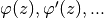 .
.spat_symbol – Sympy symbol for the spatial variable
 .
.spatial_domain (tuple) – Domain on which
is defined
(e.g.: spatial_domain=(0, 1)).complex (bool) – If False the Function raises an Error if it returns complex values. Default: False.
-
class
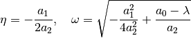
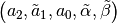
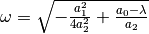
SecondOrderDirichletEigenfunction(om, param, l, scale=1, max_der_order=2)¶ Bases:
pyinduct.eigenfunctions.SecondOrderEigenfunctionThis class provides an eigenfunction
to eigenvalue
problems of the form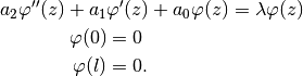
The eigenfrequency
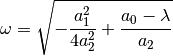
must be provided (for example with the
eigfreq_eigval_hint()of this class).- Parameters
om (numbers.Number) – eigenfrequency

param (array_like) –
l (numbers.Number) – End of the domain
.scale (numbers.Number) – Factor to scale the eigenfunctions.
max_der_order (int) – Number of derivative handles that are needed.
-
static
eigfreq_eigval_hint(param, l, n_roots)¶ Return the first n_roots eigenfrequencies
and
eigenvalues  .
.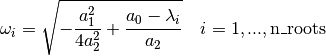
to the considered eigenvalue problem.
- Parameters
param (array_like) –
l (numbers.Number) – Right boundary value of the domain
![[0,l]\ni z](../_images/math/ab2e9c5c8aecd442ed77335337ca99f79ba220e0.png) .
.n_roots (int) – Amount of eigenfrequencies to be compute.
- Returns
![\Big(\big[\omega_1,...,\omega_\text{n\_roots}\Big],
\Big[\lambda_1,...,\lambda_\text{n\_roots}\big]\Big)](../_images/math/713cc8c64f0af1db14cd2b0b86da21c34ced44ac.png)
- Return type
tuple –> two numpy.ndarrays of length n_roots
-
class
SecondOrderEigenVector(char_pair, coefficients, domain, derivative_order)¶ Bases:
pyinduct.shapefunctions.ShapeFunctionThis class provides eigenvectors of the form

of a linear second order spatial operator
 denoted by
where the
 are constant and whose boundary conditions are given
by
are constant and whose boundary conditions are given
by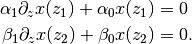
To calculate the corresponding eigenvectors, the problem
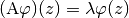
is solved for the eigenvalues
, making use of the
characteristic roots  given by
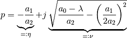
Note
To easily instantiate a set of eigenvectors for a certain system, use the
cure_hint()of this class or even better the helper-functioncure_interval().- Warns
Since an eigenvalue corresponds to a pair of conjugate complex
characteristic roots, latter are only calculated for the positive
half-plane since the can be mirrored.
To obtain the orthonormal properties of the generated
eigenvectors, the eigenvalue corresponding to the characteristic
root 0+0j is ignored, since it leads to the zero function.
- Parameters
char_pair (tuple of complex) – Characteristic root, corresponding to the eigenvalue
for which the eigenvector is
to be determined.
(Can be obtained by convert_to_characteristic_root())coefficients (tuple) – Constants of the exponential ansatz solution.
- Returns
The eigenvector.
- Return type
-
static
calculate_eigenvalues(domain, params, count, extended_output=False, **kwargs)¶ Determine the eigenvalues of the problem given by parameters defined on domain .
- Parameters
domain (
Domain) – Domain of the spatial problem.params (bunch-like) – Parameters of the system, see
__init__()for details on their definition. Long story short, it must contain .
.count (int) – Amount of eigenvalues to generate.
extended_output (bool) – If true, not only eigenvalues but also the corresponding characteristic roots and coefficients of the eigenvectors are returned. Defaults to False.
- Keyword Arguments
debug (bool) – If provided, this parameter will cause several debug windows to open.
- Returns
- , ordered in increasing
order or tuple of (
 )
if extended_output is True.
)
if extended_output is True. - Return type
array or tuple of arrays
-
static
convert_to_characteristic_root(params, eigenvalue)¶ Converts a given eigenvalue
into a
characteristic root by using the provided
parameters. The relation is given by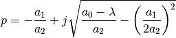
- Parameters
params (bunch) – system parameters, see
cure_hint().eigenvalue (real) – eigenvalue
- Returns
characteristic root
- Return type
complex number
-
static
convert_to_eigenvalue(params, char_roots)¶ Converts a pair of characteristic roots
 into an
eigenvalue by using the provided parameters.
The relation is given by
into an
eigenvalue by using the provided parameters.
The relation is given by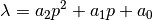
- Parameters
params (
SecondOrderOperator) – System parameters.char_roots (tuple or array of tuples) – Characteristic roots
-
static
cure_interval(interval, params, count, derivative_order, **kwargs)¶ Helper to cure an interval with eigenvectors.
- Parameters
interval (
Domain) – Domain of the spatial problem.params (
SecondOrderOperator) – Parameters of the system, see__init__()for details on their definition. Long story short, it must contain .
.count (int) – Amount of eigenvectors to generate.
derivative_order (int) – Amount of derivative handles to provide.
kwargs – will be passed to
calculate_eigenvalues()
- Keyword Arguments
debug (bool) – If provided, this parameter will cause several debug windows to open.
- Returns
An array holding the eigenvalues paired with a basis spanned by the eigenvectors.
- Return type
tuple of (array,
Base)
-
class
SecondOrderEigenfunction(*args, **kwargs)¶ Bases:
pyinduct.shapefunctions.ShapeFunctionWrapper for all eigenvalue problems of the form

with eigenfunctions
 and eigenvalues .
The roots of the characteristic equation (belonging to the ode) are denoted
by
and eigenvalues .
The roots of the characteristic equation (belonging to the ode) are denoted
by
In the following the variable
is called an eigenfrequency.-
classmethod
cure_interval(cls, interval, param=None, n=None, eig_val=None, eig_freq=None, max_order=2, scale=None)¶ Provide the first n eigenvalues and eigenfunctions (wraped inside a pyinduct base). For the exact formulation of the considered eigenvalue problem, have a look at the docstring from the eigenfunction class from which you will call this method.
You must call this classmethod with one and only one of the kwargs:
n (eig_val and eig_freq will be computed with the
eigfreq_eigval_hint())eig_val (eig_freq will be calculated with
eigval_tf_eigfreq())eig_freq (eig_val will be calculated with
eigval_tf_eigfreq()),
or (and) pass the kwarg scale (then n is set to len(scale)). If you have the kwargs eig_val and eig_freq already calculated then these are preferable, in the sense of performance.
- Parameters
interval (
Domain) – Domain/Interval of the eigenvalue problem.- Keyword Arguments
param – Parameters
 see
evp_class.__doc__.
see
evp_class.__doc__.n – Number of eigenvalues/eigenfunctions to compute.
eig_freq (array_like) – Pass your own choice of eigenfrequencies here.
eig_val (array_like) – Pass your own choice of eigenvalues here.
max_order – Maximum derivative order which must provided by the eigenfunctions.
scale (array_like) – Here you can pass a list of values to scale the eigenfunctions.
- Returns
eigenvalues (numpy.array)
eigenfunctions (
Base)
- Return type
tuple
-
static
eigfreq_eigval_hint(param, l, n_roots)¶ - Parameters
param (array_like) – Parameters
 .
.l – End of the domain
![z\in[0, 1]](../_images/math/92ae6b72d1ddc8f0340f4f3742d292008c578bb0.png) .
.n_roots (int) – Number of eigenfrequencies/eigenvalues to be compute.
- Returns
Booth tuple elements are numpy.ndarrays of the same length, one for eigenfrequencies and one for eigenvalues.
- Return type
tuple
-
static
eigval_tf_eigfreq(param, eig_val=None, eig_freq=None)¶ Provide corresponding of eigenvalues/eigenfrequencies for given eigenfreqeuncies/eigenvalues, depending on which type is given.
respectively
- Parameters
param (array_like) – Parameters
.eig_val (array_like) – Eigenvalues
.eig_freq (array_like) – Eigenfrequencies
.
- Returns
Eigenfrequencies
or eigenvalues
.- Return type
numpy.array
-
static
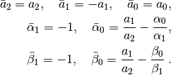
get_adjoint_problem(param)¶ Return the parameters of the adjoint eigenvalue problem for the given parameter set. Hereby, dirichlet or robin boundary condition at


and dirichlet or robin boundary condition at


can be imposed.
- Parameters
param (array_like) –
To define a homogeneous dirichlet boundary condition set alpha or beta to None at the corresponding side. Possibilities:
 ,
, ,
, or
or- .
- Returns
Parameters
 for
the adjoint problem
for
the adjoint problem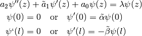
with
- Return type
tuple
-
classmethod
-
class
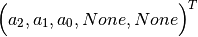
SecondOrderOperator(a2=0, a1=0, a0=0, alpha1=0, alpha0=0, beta1=0, beta0=0, domain=- np.inf, np.inf)¶ Interface class to collect all important parameters that describe a second order ordinary differential equation.
- Parameters
a2 (Number or callable) – coefficient
 .
.a1 (Number or callable) – coefficient
 .
.a0 (Number or callable) – coefficient
 .
.alpha1 (Number) – coefficient
 .
.alpha0 (Number) – coefficient
 .
.beta1 (Number) – coefficient
 .
.beta0 (Number) – coefficient
 .
.
-
static
from_dict(param_dict, domain=None)
-
static
from_list(param_list, domain=None)
-
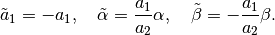
get_adjoint_problem(self)¶ Return the parameters of the operator
 describing the
the problem
describing the
the problem
where the
 are constant and whose boundary conditions
are given by
are constant and whose boundary conditions
are given by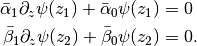
The following mapping is used:
- Returns
Parameter set describing
.- Return type
-
class
SecondOrderRobinEigenfunction(om, param, l, scale=1, max_der_order=2)¶ Bases:
pyinduct.eigenfunctions.SecondOrderEigenfunctionThis class provides an eigenfunction
to the eigenvalue
problem given by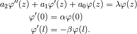
The eigenfrequency
 must be provided (for example with the
 eigfreq_eigval_hint()of this class).- Parameters
om (numbers.Number) – eigenfrequency
param (array_like) –
l (numbers.Number) – End of the domain
.scale (numbers.Number) – Factor to scale the eigenfunctions (corresponds to
 ).
).max_der_order (int) – Number of derivative handles that are needed.
-
static
eigfreq_eigval_hint(param, l, n_roots, show_plot=False)¶ Return the first n_roots eigenfrequencies
and
eigenvalues .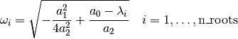
to the considered eigenvalue problem.
- Parameters
param (array_like) – Parameters
l (numbers.Number) – Right boundary value of the domain
.n_roots (int) – Amount of eigenfrequencies to compute.
show_plot (bool) – Show a plot window of the characteristic equation.
- Returns
![\Big(\big[\omega_1, \dotsc, \omega_{\text{n\_roots}}\Big],
\Big[\lambda_1, \dotsc, \lambda_{\text{n\_roots}}\big]\Big)](../_images/math/25aa66a7397d6151f3157a245c1e7995d59d6981.png)
- Return type
tuple –> booth tuple elements are numpy.ndarrays of length nroots
-
class
ShapeFunction(*args, **kwargs)¶ Bases:
pyinduct.core.FunctionBase class for approximation functions with compact support.
When a continuous variable of e.g. space and time
 is
decomposed in a series
is
decomposed in a series
 the
the  denote the shape functions.
-
classmethod
cure_interval(cls, interval, **kwargs)¶ Create a network or set of functions from this class and return an approximation base (
Base) on the given interval.The
kwargsmay hold the order of approximation or the amount of functions to use. Use them in your child class as needed.If you don’t need to now from which class this method is called, overwrite the
@classmethoddecorator in the child class with the@staticmethoddecorator.Short reference: Inside a
@staticmethodyou know nothing about the class from which it is called and you can just play with the given parameters. Inside a@classmethodyou can additionally operate on the class, since the first parameter is always the class itself.
-
classmethod
-
class
TransformedSecondOrderEigenfunction(target_eigenvalue, init_state_vector, dgl_coefficients, domain)¶ Bases:
pyinduct.core.FunctionThis class provides an eigenfunction
to the eigenvalue
problem given by
where
 denotes an eigenvalue and
![z \in [z_0, \dotsc, z_n]](../_images/math/984b557643c06e38e8ebd13c6e7a7507848dc659.png) the domain.
the domain.- Parameters
target_eigenvalue (numbers.Number) –
init_state_vector (array_like) –
dgl_coefficients (array_like) – Function handles
 .
.domain (
Domain) – Spatial domain of the problem.
-
find_roots(function, grid, n_roots=None, rtol=1e-05, atol=1e-08, cmplx=False, sort_mode='norm')¶ Searches n_roots roots of the function
 on the given grid and checks them for uniqueness with aid of rtol.
In Detail
scipy.optimize.root()is used to find initial candidates for roots of . If a root satisfies the criteria
given by atol and rtol it is added. If it is already in the list,
a comprehension between the already present entries’ error and the
current error is performed. If the newly calculated root comes
with a smaller error it supersedes the present entry.- Raises
ValueError – If the demanded amount of roots can’t be found.
- Parameters
function (callable) – Function handle for math:f(boldsymbol{x}) whose roots shall be found.
grid (list) – Grid to use as starting point for root detection. The
 th element of this list provides sample points
for the th parameter of
th element of this list provides sample points
for the th parameter of  .
.n_roots (int) – Number of roots to find. If none is given, return all roots that could be found in the given area.
rtol – Tolerance to be exceeded for the difference of two roots to be unique:
 .
.atol – Absolute tolerance to zero:
 .
.cmplx (bool) – Set to True if the given function is complex valued.
sort_mode (str) – Specify tho order in which the extracted roots shall be sorted. Default “norm” sorts entries by their
 norm,
while “component” will sort them in increasing order by every
component.
norm,
while “component” will sort them in increasing order by every
component.
- Returns
numpy.ndarray of roots; sorted in the order they are returned by
.
-
generic_scalar_product(b1, b2=None, scalar_product=None)¶ Calculates the pairwise scalar product between the elements of the
ApproximationBaseb1 and b2.- Parameters
b1 (
ApproximationBase) – first basisb2 (
ApproximationBase) – second basis, if omitted defaults to b1scalar_product (list of callable) – Callbacks for product calculation. Defaults to scalar_product_hint from b1.
Note
If b2 is omitted, the result can be used to normalize b1 in terms of its scalar product.
-
normalize_base(b1, b2=None)¶ Takes two
ApproximationBase’s ,
and normalizes them so that
,
and normalizes them so that
 .
If only one base is given,
.
If only one base is given,  defaults to .
- Parameters
b1 (
ApproximationBase) –b2 (
ApproximationBase) –
- Raises
ValueError – If
and are orthogonal.- Returns
if b2 is None, otherwise: Tuple of 2
ApproximationBase’s.- Return type
ApproximationBase
-
real(data)¶ Check if the imaginary part of
datavanishes and return its real part if it does.- Parameters
data (numbers.Number or array_like) – Possibly complex data to check.
- Raises
ValueError – If provided data can’t be converted within the given tolerance limit.
- Returns
Real part of
data.- Return type
numbers.Number or array_like
-
visualize_roots(roots, grid, func, cmplx=False, return_window=False)¶ Visualize a given set of roots by examining the output of the generating function.
- Parameters
roots (array like) – Roots to display, if None is given, no roots will be displayed, this is useful to get a view of func and choosing an appropriate grid.
grid (list) – List of arrays that form the grid, used for the evaluation of the given func.
func (callable) – Possibly vectorial function handle that will take input of of the shape (‘len(grid)’, ).
cmplx (bool) – If True, the complex valued func is handled as a vectorial function returning [Re(func), Im(func)].
return_window (bool) – If True the graphics window is not shown directly. In this case, a reference to the plot window is returned.
Returns: A PgPlotWindow if delay_exec is True.