Control¶

class IntegralTerm(integrand, limits, scale=1.0)¶

Bases: pyinduct.placeholder.EquationTerm

Class that represents an integral term in a weak equation.

Parameters

integrand –
limits (tuple) –
scale –

class ScalarTerm(argument, scale=1.0)¶

Bases: pyinduct.placeholder.EquationTerm

Class that represents a scalar term in a weak equation.

Parameters

argument –
scale –

class SimulationInput(name='')¶

Bases: object

Base class for all objects that want to act as an input for the time-step simulation.

The calculated values for each time-step are stored in internal memory and can be accessed by get_results() (after the simulation is finished).

Note

Due to the underlying solver, this handle may get called with time arguments, that lie outside of the specified integration domain. This should not be a problem for a feedback controller but might cause problems for a feedforward or trajectory implementation.

clear_cache(self)¶

Clear the internal value storage.

When the same SimulationInput is used to perform various simulations, there is no possibility to distinguish between the different runs when get_results() gets called. Therefore this method can be used to clear the cache.

get_results(self, time_steps, result_key='output', interpolation='nearest', as_eval_data=False)¶

Return results from internal storage for given time steps.

Raises

Error – If calling this method before a simulation was run.

Parameters

time_steps – Time points where values are demanded.
result_key – Type of values to be returned.
interpolation – Interpolation method to use if demanded time-steps are not covered by the storage, see scipy.interpolate.interp1d() for all possibilities.
as_eval_data (bool) – Return results as EvalData object for straightforward display.

Returns

Corresponding function values to the given time steps.

class SimulationInputSum(inputs)¶

Bases: pyinduct.simulation.SimulationInput

Helper that represents a signal mixer.

class StateFeedback(control_law)¶

Bases: pyinduct.feedback.Feedback

Base class for all feedback controllers that have to interact with the simulation environment.

Parameters: control_law (WeakFormulation) – Variational formulation of the control law.

class WeakFormulation(terms, name, dominant_lbl=None)¶

Bases: object

This class represents the weak formulation of a spatial problem. It can be initialized with several terms (see children of EquationTerm). The equation is interpreted as

$term_0 + term_1 + ... + term_N = 0.$

Parameters

terms (list) – List of object(s) of type EquationTerm.
name (string) – Name of this weak form.
dominant_lbl (string) – Name of the variable that dominates this weak form.

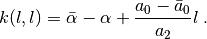
get_parabolic_robin_backstepping_controller(state, approx_state, d_approx_state, approx_target_state, d_approx_target_state, integral_kernel_ll, original_beta, target_beta, scale=None)¶

Build a modal approximated backstepping controller 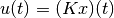$u(t)=(Kx)(t)$ , for the (open loop-) diffusion system with reaction term, robin boundary condition and robin actuation

$\begin{align*} \dot x(z,t) &= a_2 x''(z,t) + a_0 x(z,t), && z\in (0, l) \\ x'(0,t) &= \alpha x(0,t) \\ x'(l,t) &= -\beta x(l,t) + u(t) \end{align*}$

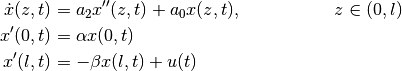
such that the closed loop system has the desired dynamic of the target system

$\begin{align*} \dot{\bar{x}}(z,t) &= a_2 \bar x''(z,t) + \bar a_0 \bar x(z,t), && z\in (0, l) \\ \bar x'(0,t) &= \bar\alpha \bar x(0,t) \\ \bar x'(l,t) &= -\bar\beta x(l,t) \end{align*}$

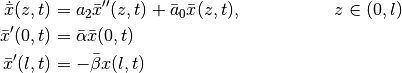
where $\bar a_0,\, \bar\alpha,\, \bar\beta$ are controller parameters.

The control design is performed using the backstepping method, whose integral transform

$\bar x(z) = x(z) + \int_0^z k(z, \bar z) x(\bar z) \, d\bar z$

maps from the original system to the target system.

Note

For more details see the example script pyinduct.examples.rad_eq_const_coeff that implements the example from [WoiEtAl17] .

Parameters

state (list of ScalarTerm’s) – Measurement / value from simulation of $x(l)$ .
approx_state (list of ScalarTerm’s) – Modal approximated $x(l)$ .
d_approx_state (list of ScalarTerm’s) – Modal approximated $x'(l)$ .
approx_target_state (list of ScalarTerm’s) – Modal approximated $\bar x(l)$ .
d_approx_target_state (list of ScalarTerm’s) – Modal approximated $\bar x'(l)$ .
integral_kernel_ll (numbers.Number) –
Integral kernel evaluated at $\bar z = z = l$ :

$k(l, l) = \bar\alpha - \alpha + \frac{a_0-\bar a_0}{a_2} l \:.$
original_beta (numbers.Number) – Coefficient $\beta$ of the original system.
target_beta (numbers.Number) – Coefficient $\bar\beta$ of the target system.
scale (numbers.Number) – A constant $c \in \mathbb R$ to scale the control law: $u(t) = c \, (Kx)(t)$ .

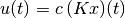Returns

$(Kx)(t)$

Return type

StateFeedback

WoiEtAl17: Frank Woittennek, Marcus Riesmeier and Stefan Ecklebe; On approximation and implementation of transformation based feedback laws for distributed parameter systems; IFAC World Congress, 2017, Toulouse

scale_equation_term_list(eqt_list, factor)¶

Temporary function, as long EquationTerm can only be scaled individually.

Parameters

eqt_list (list) – List of EquationTerm’s
factor (numbers.Number) – Scale factor.

Returns

Scaled copy of EquationTerm’s (eqt_list).

split_domain(n, a_desired, l, mode='coprime')¶

Consider a domain $[0,l]$ which is divided into the two sub domains $[0,a]$ and $[a,l]$ with the discretization $l_0 = l/n$ and a partition $a + b = l$ .

Calculate two numbers $k_1$ and $k_2$ with $k_1 + k_2 = n$ such that $n$ is odd and $a = k_1l_0$ is close to a_desired.

Parameters

n (int) – Number of sub-intervals to create (must be odd).
a_desired (float) – Desired partition size $a$ .
l (float) – Length $l$ of the interval.
mode (str) –
Operation mode to use:
- ’coprime’: $k_1$ and $k_2$ are coprime (default) .
- ’force_k2_as_prime_number’: $k_2$ is a prime number ( $k_1$ and $k_2$ are coprime)
- ’one_even_one_odd’: One is even and one is odd.