Feedforward
-
class
InterpolationTrajectory(t, u, **kwargs)¶ Bases:
pyinduct.simulation.SimulationInputProvides a system input through one-dimensional linear interpolation in the given vector
 .
.- Parameters
t (array_like) – Vector
 with time steps.
u (array_like) – Vector
with function values, evaluated at .**kwargs – see below
- Keyword Arguments
show_plot (bool) – to open a plot window, showing u(t).
scale (float) – factor to scale the output.
-
get_plot(self)¶ Create a plot of the interpolated trajectory.
Todo
the function name does not really tell that a QtEvent loop will be executed in here
- Returns
the PlotWindow widget.
- Return type
(pg.PlotWindow)
-
scale(self, scale)
-
class
RadFeedForward(l, T, param_original, bound_cond_type, actuation_type, n=80, sigma=None, k=None, length_t=None, y_start=0, y_end=1, **kwargs)¶ Bases:
pyinduct.trajectory.InterpolationTrajectoryClass that implements a flatness based control approach for the reaction-advection-diffusion equation

with the boundary condition
bound_cond_type == "dirichlet":
A transition from
 to
to  is
considered.
is
considered.With
 where
where  is the flat output.
bound_cond_type == "robin":
A transition from
 to
to  is
considered.
is
considered.With
 where is the flat output.
and the actuation
actuation_type == "dirichlet":
actuation_type == "robin": .
.
The flat output trajectory
will be calculated with
gevrey_tanh().- Parameters
l (float) – Domain length.
t_end (float) – Transition time.
param_original (tuple) – Tuple holding the coefficients of the pde and boundary conditions.
bound_cond_type (string) – Boundary condition type. Can be dirichlet or robin, see above.
actuation_type (string) – Actuation condition type. Can be dirichlet or robin, see above.
n (int) – Derivative order to provide (defaults to 80).
sigma (number.Number) – sigma value for
gevrey_tanh().k (number.Number) – K value for
gevrey_tanh().length_t (int) – length_t value for
gevrey_tanh().y0 (float) – Initial value for the flat output.
y1 (float) – Desired value for the flat output after transition time.
**kwargs – see below. All arguments that are not specified below are passed to
InterpolationTrajectory.
-
class
SecondOrderOperator(a2=0, a1=0, a0=0, alpha1=0, alpha0=0, beta1=0, beta0=0, domain=- np.inf, np.inf)¶ Interface class to collect all important parameters that describe a second order ordinary differential equation.
- Parameters
a2 (Number or callable) – coefficient
 .
.a1 (Number or callable) – coefficient
 .
.a0 (Number or callable) – coefficient
 .
.alpha1 (Number) – coefficient
 .
.alpha0 (Number) – coefficient
 .
.beta1 (Number) – coefficient
 .
.beta0 (Number) – coefficient
 .
.
-
static
from_dict(param_dict, domain=None)
-
static
from_list(param_list, domain=None)
-
get_adjoint_problem(self)¶ Return the parameters of the operator
 describing the
the problem
describing the
the problem
where the
 are constant and whose boundary conditions
are given by
are constant and whose boundary conditions
are given by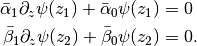
The following mapping is used:
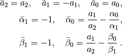
- Returns
Parameter set describing
.- Return type
-
eliminate_advection_term(param, domain_end)¶ This method performs a transformation
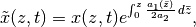
on the system, which eliminates the advection term
 from a
reaction-advection-diffusion equation of the type:
from a
reaction-advection-diffusion equation of the type:
The boundary can be given by robin

dirichlet

or mixed boundary conditions.
- Parameters
param (array_like) –
domain_end (float) – upper bound of the spatial domain
- Raises
TypeError – If
 is callable but no derivative handle is
defined for it. –
- Returns
Parameters
the transformed system

and the corresponding boundary conditions (
 and/or
 set to None by dirichlet boundary condition).
- Return type
SecondOrderOperator or tuple
-
gevrey_tanh(T, n, sigma=1.1, K=2, length_t=None)¶ Provide Gevrey function
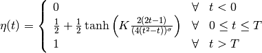
with the Gevrey-order
 and the derivatives
up to order n.
and the derivatives
up to order n.Note
For details of the recursive calculation of the derivatives see:
Rudolph, J., J. Winkler und F. Woittennek: Flatness Based Control of Distributed Parameter Systems: Examples and Computer Exercises from Various Technological Domains (Berichte aus der Steuerungs- und Regelungstechnik). Shaker Verlag GmbH, Germany, 2003.
- Parameters
T (numbers.Number) – End of the time domain=[0, T].
n (int) – The derivatives will calculated up to order n.
sigma (numbers.Number) – Constant
 to adjust the Gevrey
order of
to adjust the Gevrey
order of  .
.K (numbers.Number) – Constant to adjust the slope of
.length_t (int) – Ammount of sample points to use. Default:
int(50 * T)
- Returns
numpy.array([[
], … , [ ]])
]])t: numpy.array([0,…,T])
- Return type
tuple
-
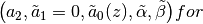
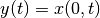
power_series_flat_out(z, t, n, param, y, bound_cond_type)¶ Provides the solution
 (and the spatial derivative
 ) of the pde
as power series approximation:
for the boundary condition (
bound_cond_type == "dirichlet") and the flat output 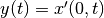 with
with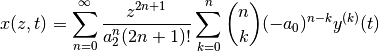
for the boundary condition (
bound_cond_type == "robin") and the flat output
 with
with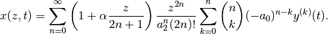
- Parameters
z (array_like) –
![[0, ..., l]](../../_images/math/be97c3cc534571ef8e5c4b073bbc91a325778ac4.png)
t (array_like) –
![[0, ... , T]](../../_images/math/d673c59a7a9fd4a179936bbb75b31b8e63ee7b44.png)
n (int) – Series termination index.
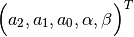
param (array_like) –
Parameters
![[a_2, a_1, a_0, \alpha, \beta]](../../_images/math/2acc97bb56ef983557ba4980581b6491c1f7793d.png)
 for
for bound_cond_type == dirichlet is not used from this function
but has to be provided (for now)
is not used from this function
but has to be provided (for now)
y (array_like) –
Flat output
and derivatives:![[[y(0), ..., y(T)],...,[y^{(n/2)}(0), ..., y^{(n/2)}(T)]].](../../_images/math/568ce6e9736b7af83763255f687a6c19d3064919.png)
bound_cond_type (str) –
dirichletorrobin
- Returns
Solution
of the pde and the spatial derivative
.- Return type
tuple